The data used in this study were collected as part of a statewide insecticide resistance monitoring effort that is described in detail in Estep et al. 2018. The frequencies of kdr genotypes were determined for Ae. aegypti strains collected as eggs or larvae at 62 sites across 18 counties, primarily in 2016 and 2017, although Ae. aegypti from one site (Hillsborough County) were collected in 2014. For 21 sites, specimens from collections in close proximity to each other were pooled to the geographic mean center of the contributing locations (Figure 1).
We used the weighted Ripley’s K-function to characterize spatial dependency in the recorded frequencies of the resistant IICC genotype across the 62 sampled sites in Florida. The Ripley’s K-function summarizes the extent to which points are clustered or dispersed across a range of distance bands (26). This is done by comparing the actual number of neighboring points present within a circle centered on an arbitrary point to the number of points that would be expected given a random distribution. In a weighted K-function analysis, the null hypothesis is that the pattern of weight values (in this case, the frequency of the IICC genotype) assigned to the points is not significantly more clustered than the underlying pattern of the points. This analysis was implemented in ArcMap 10.6 with 30 distance bands of 5 kilometers. A minimum enclosing rectangle, which is the smallest rectangle that can be generated to include all the sampling sites, was used as the study area for the analysis. This was chosen as an alternative to using the Florida boundaries, since sampling was not evenly distributed throughout the state and was not conducted at all in the Florida Panhandle. The Ripley’s edge correction formula was applied to account for points located near the edge of the study area. The confidence interval was computed based on 999 permutations of random point patterns, derived from the first implementation of the Ripley’s K-function on the unweighted sampling sites, while the plot of observed spatial dependency was based on the sampling sites, weighted by the frequency of the IICC genotype.
We used SaTScan Version 9.4 (27) to identify and map clusters of the different kdr genotypes. This software detects clusters in space and time and tests identified clusters for statistical significance. We used the multinomial probability model (28), allowing detection of higher or lower than expected frequencies of each unique kdr genotype, and implemented both a circular and elliptical window shape to allow comparisons between the two methods (29). The genotype frequencies, which ranged from 0.0 to 1.0 in the original dataset, were multiplied by 100 and rounded to the nearest integer, then imported as case counts. The population for each site was set to 100 individuals. After experimentation at different maximum spatial cluster sizes, 15% of the population at risk was used as the cut-off value. This maximum cluster size detected clusters at scales that approximated the county-level scale of vector control implementation, whereas larger thresholds yielded clusters that encompassed many counties, and smaller thresholds resulted in many clusters that only included a single site. We used 999 standard Monte Carlo replications to compute significance and allowed adjustment for more likely clusters.
Several landscape variables were considered as potential covariates in the model of pyrethroid-resistant IICC genotype frequency (Table 1). Products derived from the Moderate Resolution Imaging Spectroradiometer (MODIS) were downloaded to represent vegetation density. This included the MODIS Vegetation Continuous Fields products, which are generated annually based on monthly composites to represent percent tree cover and percent non-tree vegetation cover at a scale of 250 meters (30). MODIS-derived enhanced vegetation index (EVI) and leaf area index (LAI) products were also included, representing vegetation conditions in January, April, July, and October 2016. Because vector control districts frequently apply insecticides from ground vehicles in Florida, we also included spatial data representing the configuration of road networks. The 2016 TIGER/Line road files were downloaded from the United States Census Bureau (31), and Euclidean distance and road density were calculated using the dataset of only primary and secondary roads as well as the dataset of all roads. To represent agricultural land use, we downloaded the 2016 United States Department of Agriculture National Cropland Data Layer and calculated the Euclidean distance from all agricultural land cover and from each of the five most abundant crop types in Florida (oranges, sugar cane, hay, peanuts, and cotton) (32). We also included data on land cover and percent impervious surface from the 2016 National Land Cover Database, published by the Multi-Resolution Land Characteristics Consortium (33). Euclidean distances from urban or built-up land, forested land, and wetland were calculated for the study area. Finally, we included data on the 5-year estimates of median household income and population density at the census tract level from the United States Census Bureau 2016 American Community Survey (34).
All of the spatial data described above were projected to the Albers Conic Equal Area projection used by the Florida Geographic Data Library, clipped to the state boundary, and resampled to 250 m resolution, which was the coarsest spatial resolution of the input datasets. We extracted values from each dataset at the sampling site locations. In cases where multiple neighboring sites were pooled to a centroid, we generated a single standard deviation ellipse centered on the centroid to capture the dispersal of the contributing sites,and calculated the mean value for the pixels included within the ellipse.
In addition to landscape factors, we included information on insecticide use by vector control districts in 2016. Each vector control district in the state submits an annual Chemical Activity Report to the Florida Department of Agriculture and Consumer Services (FDACS), detailing the types and amounts of adulticides and larvicides used, as well as the number of acres treated. We summarized adulticide use by class as gallons of active ingredient used per acre treated for each district. We also calculated the combined amount of adulticides used in each district as the total number of gallons of active ingredient per acre treated.
We used a beta regression modelling framework to test for statistically significant associations between the variables described above and the frequency of the IICC genotype in collected Ae. aegypti specimens. Beta regression was selected because it is an appropriate model in cases where the dependent variable is a proportion ranging from 0 to 1, as was the case for the IICC genotype frequency (35). Prior to implementing the model, the distributions of all explanatory variables were assessed for approximate normality using density plots and log transformed as necessary, and each individual predictor was plotted against the response variable to determine if a linear relation would likely be appropriate. All explanatory variables were rescaled to have a mean of zero and a standard deviation of one, due to the wide-ranging scales of measurement used across the original, unscaled set of variables (36). To assess for collinearity between the explanatory variables, we used variance inflation factors (VIF), calculated with the ‘vifstep’ function with a threshold of 10 using the “USDM” R package (37). Ten variables were removed based on this threshold, and the remaining 22 variables were included in the full model, generated using the “betareg” R package (38). All potential combinations of variables were considered using the dredge function in the “MuMIn” R package, with a limit of six explanatory variables (39). The models were ranked by AICc, a variant of Akaike’s Information Criterion that is adjusted for small sample sizes, and the twenty best-performing models by this metric were considered.
Table 1. Variables considered for beta regression models and data source
|
Variable
|
Source
|
Date
|
|
Distance from agricultural land
|
National Cropland Data Layer
|
2016
|
|
Distance from oranges, sugar cane
|
|
Distance from sugar production
|
|
Distance from hay production
|
|
Distance from peanut production
|
|
Distance from cotton production
|
|
Primary and secondary road density
|
United States Census Bureau TIGER Shapefiles
|
2016
|
|
Distance from primary and secondary road
|
|
All roads density
|
|
Distance from all roads
|
|
Percent tree cover
|
MODIS Vegetation Continuous Fields
|
2016
|
|
Percent non-tree vegetation cover
|
|
16-day composite of enhanced vegetation index (EVI)*
|
MODIS LP DAAC
|
2016
|
|
16-day composite of leaf area index (LAI)**
|
|
Distance from urban or built-up land cover
|
National Land Cover Database
|
2016
|
|
Distance from forest land
|
|
Distance from wetland
|
|
Percent impervious surface
|
|
Population density
|
United States Census Bureau American Community Survey
|
2016
|
|
Median household income
|
|
Pyrethroid use by control district
Organophosphate use by control district
Total insecticide use by control district
|
Florida Department of Agriculture and Consumer Services
|
2016
|
*EVI 17 January 2016, 22 April 2016, 27 July 2016, 15 October 2016; **LAI 24 January 2016, 30 April 2016, 24 July 2016, 23 October 2016.
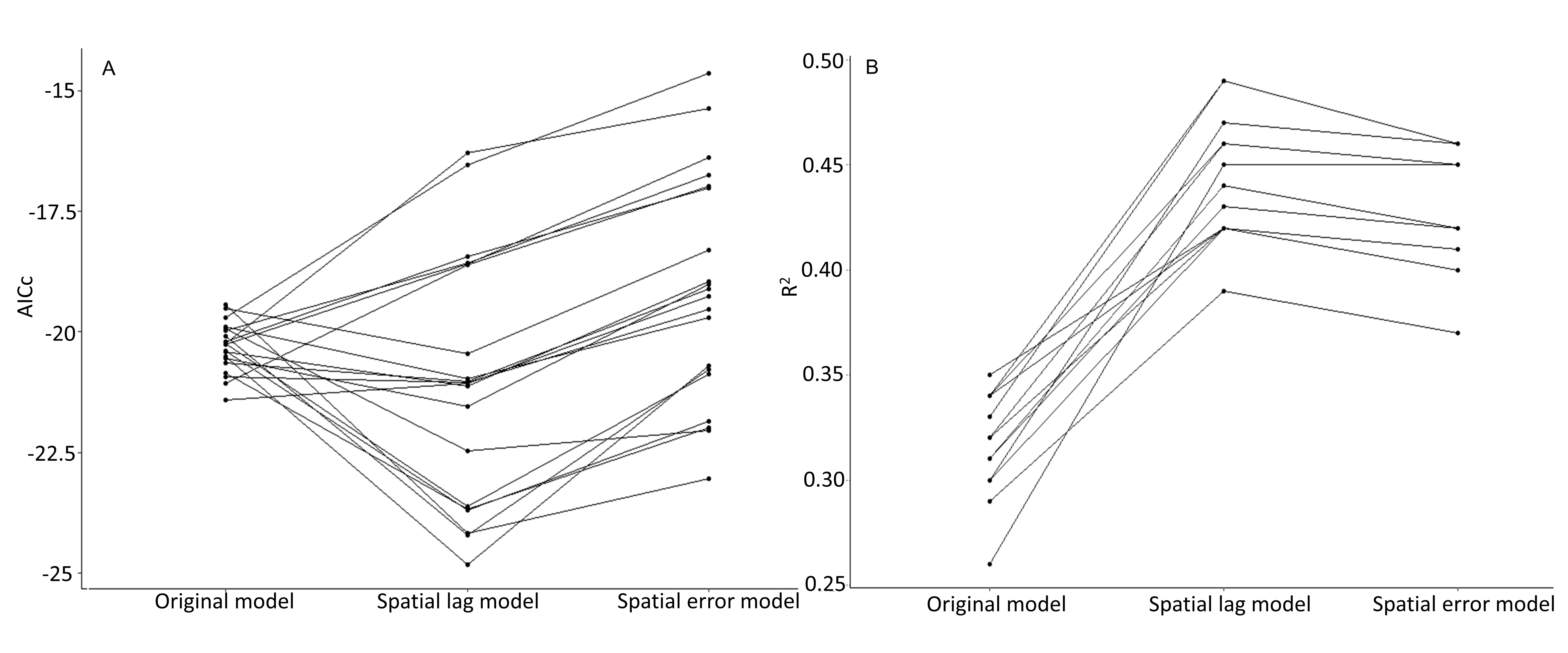
We assessed the top ten models using standard regression diagnostics and tested the residual values from these models for spatial autocorrelation using the Moran’s I statistic, with a k-nearest neighbors weights matrix. We used three nearest neighbors instead of a distance-based weights matrix due to the underlying, clustered distribution of the sampling sites. When considering alternative weights matrices, smaller distances resulted in outlying sites being without neighbors, while larger distances resulted in most of the sampling locations being neighbors for more central sites. We considered spatial lag and spatial error models, using the “spdep” R package (40), comparing them to the original models using likelihood-ratio (LR) tests, Wald tests, AICc, and pseudo R2 values.