Performance of our virtual barcode
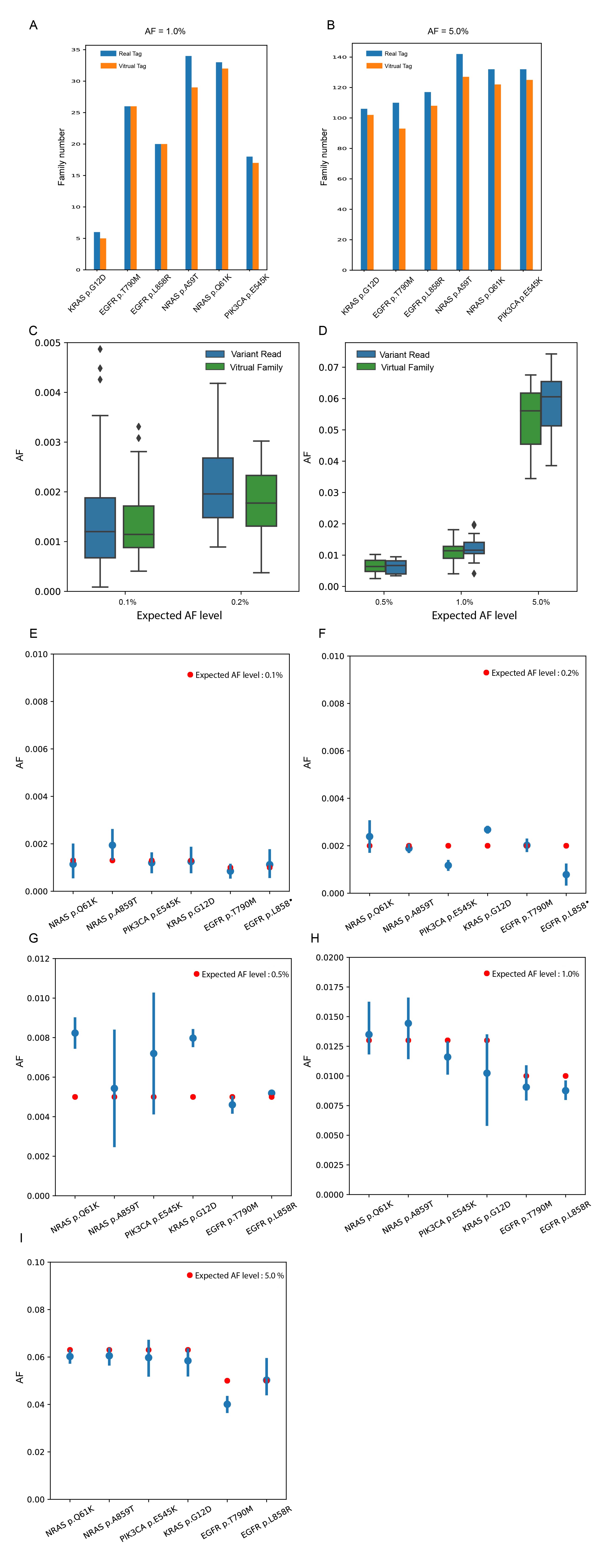
The real family was clustered by UMI, start site and template length. The virtual family was defined as reads that shared the same start site, template length and strand. The mean virtual family numbers were slightly fewer than the mean real family numbers (2730 vs. 2943) (Figure 2A, red bar vs. yellow bar) among 10 samples, and a strong linear relationship was found between virtual and real family numbers among 20000 randomly selected genomic positions in one sample (Figure 2B; y=1.105x - 75.152, 95% Confidence interval (CI): 1.1038~1.1058, P<10-40; R2=100%). The recovery rates for real families among the majority of the 20,000 positions ranged from 91.87% to 94.0% (Figure 2C; 92.98%±1.1%) and only a small proportion of reads with different UMI tags were mistakenly clustered by the virtual barcode. The incorrectly clustered family contents were investigated. The results showed that 92.6% of these members were composed of two real families, and 6.8% were three real families (Figure 2D). The incorrect clusters might introduce false negatives, particularly if the allele number of a variant is extremely low. Thus, we compared f=1.0 virtual family numbers with f=1.0 real family numbers at six positive sites among three UMI samples. At the 0.1% level, five out of the six positive sites had equal family numbers and no false negatives were detected (Figure 2E). Similar to the 1% and 5% levels, no false negatives were found (Figure S1). At the same time, AF values of six positive sites calculated from the virtual-family level were close to the expected AF values and similar to the AF values from the variant-read level (Figure S1). In the decreasing noise aspect, efficiencies of the virtual tag and real tag were the same, supported by similar mean fraction of panel-wide error-free genomic positions (Figure 2F; Real tag: 84.44%±0.91%; Virtual tag: 88.07%±0.66%) and mean panel-wide error rates (Real tag: 7.1*10-5±0.3*10-5; Virtual Tag: 5.9*10-5±0.5*10-5).
In conclusion, our virtual barcode was sufficiently robust to replace a real UMI tag and could become a universally applicable approach for reducing noise in cfDNA sequencing samples.
Subsequently, virtual barcode was applied for 30 BGs, and the panel-wide error position percentage was significantly decreased in every BG (Figure 3A). In turn, the mean panel-wide error-free position percentage was improved by ~64.11%±12.9%. The ability of the method to decrease random read errors was further confirmed at six positive sites in the top 7 high-sequencing-depth control samples. There were random non-reference alleles in two or more samples at the positive site (Figure 3B), and nearly all of these alleles were eliminated (Figure 3C). These results confirmed the good and stable performance of our virtual barcode for decreasing read-level stochastic noise.
Characteristics of mutant-family-level noise
A small proportion of error sites supported with f=1.0 mutant families made the virtual barcode/real tag alone indistinguishable from real variants. We denote this type of noise mutant-family-level noise (designated as f=1.0 sites). Thus, additional robust filters are needed to improve the specificity of the proposed algorithm.
The profiles of mutant-family-level noise among 14 controls and 16 RSDs showed an interesting divergence. A significant linear relationship between the mean depth and error position percentage (Figure 3D; y=0.347x + 0.412, 95% CI: 0.292~0.402, P=2.8*10-13; R2=85.56%) remained at the mutant-family-level in the RSDs (Figure 3E, green line; y=0.083x + 0.029, 95% CI: 0.059~0.107, P=5.22*10-6; R2 =80.82%;) but not among the controls (Figure 3E, red dots). This disagreement might be caused by input DNA quantities (virtual family numbers) and uneven depth/coverage. By normalizing panel-wide virtual family numbers based on coverage, the family degree was obtained for every sample. Compared with controls, the median virtual family degree was significantly higher in both Oncosmart2 (2.49-fold, P=2.26*10-5) and Oncosmart3 RSDs (1.88-fold, P=0.007; Figure 3F). Based on the observation that the reciprocal of family degree could reflect panel-wide median virtual family size (Figure S2), 14 controls had significantly larger overall virtual family size than 16 RSDs (Figure 3G; P=5.88*10-5), which in turn could give more confident support for calculating f values and further decreasing random read-level noise (Figure 3E; Figure S2). The significantly larger family size in 14 controls was caused by the significantly lower template numbers than 16 RSDs (P = 2.05*10-5, Figure S2). The scatterplot clearly showed that high template numbers in 16 RSDs caused a significantly higher percentage of mutant-family-level noise than 14 controls (P = 6.25*10-8; Figure 3H). This result indicated that using cfDNA data from normal healthy individuals with low-level templates as the background (20, 41) is not sufficient to cover all noises in samples with high-level templates under similar sequencing coverage. Thus, we combined controls with RSDs for the following analysis.
According to the relationship between sample occurrence and AF spectra (Figure S3), mutant-family-level noises were classified into two types: stereotypical (occurrence >=6 BGs) and stochastic mutant-family-level noise. In total, we obtained 265 unique stereotypical variants (Figure 4A). The RSDs made a greater contribution than the controls to recovering stereotypical variants, many of which occurred only once in controls (Figure S4). As expected, 265 stereotypical noises occurred stably showing a significant linear relationship between 25 Oncosmart2 BGs and 529 Oncosmart2 cfDNA samples (Figure S3; y=1.097x - 0.137, 95% CI: 0.922~1.235, P=5.6*10-32; R2=41.7%). Further analysis of the occurrence rates of 121 shared noises (Figure 4A) showed a significant linear relationship with a higher R2 value (Figure 4B; y=1.164 x – 0.187, 95% CI: 1.019 ~ 1.308, P=4.7*10-12; R2=67.8%). Additionally, after polishing based on Oncosmart2, no stereotypical noises were found among the 5 Oncosmart3 RSDs at the intersection region of the two panels (Table S2-2). Stereotypical noise is caused by many factors, such as DNA damage (42) and PCR errors (43), which have different substitution preferences. The main substitution types of our stereotypical variants were C>T/G>A, C>A/G>T, and A>G/T>C (71.05%, Figure 4C), which were consistent with the substitution types from Oncosmart3 RSDs (Table S2-4) and previously reported error profiles for ‘Kapa HF’ polymerase (43). The percentage of these six substitutions further increased to 84.297% in 121 shared sites, which demonstrated that these substitutions introduced by PCR errors were likely to occur universally (Figure 4B, Figure S3; R2:67.8% vs. 41.7%). These PCR-induced distortions are mainly caused by PCR stochasticity and polymerase errors (43, 44) and cannot be removed by UMI strategies only(20, 43).
Strategies for decreasing mutant-family-level noises
Based on a clear understanding of the characteristics of stereotypical noise, a filtered database was constructed for the polishing of real mutations of the same type at these sites (265 polishing sites). Unlike in the previously proposed iDES polishing method (20), we first obtained 10 best-fit candidate distributions from 529 Oncosmart2 cfDNA samples based on AIC, BIC, SEE, and R values, which were independently validated in 104 Oncosmart1 cfDNA samples. Then a comparison between the iDES construction step and our step was made (Figure S4). Finally, 265 stereotypical variants were polished by calculating cutoff AF values from the best-fitted personalized distribution. The results showed that the ‘Johnsonsu’ distribution was the best-fitted distribution (Table 1; 26%). AF cutoffs are shown in Table S3-3.
Compared with stereotypical noises, stochastic mutant-family-level noises (designated as stochastic f=1.0 site) were prone to low AF values, wide AF value spectra and unstable occurrence (Figure S3). Three additional fine-tuning filters were proposed based on appropriate specific features.
The minimum absolute distance (Ds value) was obtained between the distances from the variant position to the start and end positions in the corresponding virtual family. Ds trajectories of f=1.0 families from the stochastic f=1.0 site were compared with Ds trajectories from high-AF sites, positive sites, mutant singletons, and Ds trajectories of f<1.0 virtual families from genomic sites filtered by the virtual barcode step (Figure S5). Then, the specific Ds value (<=2 and >=149) for stochastic f=1.0 site was obtained. The virtual family that met the identified Ds value was defined as a false family. In every BG, the percentage of sites fully constituted by a false family (false family ratio: FFR=1.0) was calculated and is shown as an orange bar in Figure 4D and Figure S9.
With respect to the variant singleton ratio, based on the observation that variant singleton numbers (ranging from 0 to 39) among stochastic f=1.0 sites were significantly higher than variant singleton numbers among six positive sites, we hypothesized that for the real SNV site, the ratio of singleton numbers to f=1.0 family numbers would fluctuate within a certain range. First, at the panel level, the singleton ratios of all BGs were less than 2.0 (Figure 4E). This singleton ratio was a general robust cutoff value that could well distinguish positive mutations, known mutations of non-small-cell lung carcinoma (NSCLC) patients (45) and high AF variants from these stochastic family-level noises(Figure S6). Second, at the sample level, the mean variant singleton ratios of high-AF sites could reflect the panel-wide singleton ratio, indicating that the variant singleton ratios of real variants fluctuated around the panel-wide singleton ratio (Figure 4F). Thus, a sample-level strategy based on the distribution of singleton ratios from high-AF variants (AF>=0.05) was applied (Figure S6). After false discovery rate (FDR) correction, a small number (blue bar) of extreme outliners with mean ratios ranging from 4.1~28.2 (orange bar) were removed (FDR<=0.01; Figure 4G). In addition, our method was relatively conservative, and no outliers were found in samples with an overall high or low singleton ratio (Figure S6), such as two tumor samples (Figure 4G). In conclusion, this filter could avoid over-recovery of variant singletons at genomic sites vulnerable to random noise.
Finally, template numbers were updated and updated f=1.0 numbers and qualified variant singletons were obtained. This updated template feature was the most specific features (Figure S7). Based on this specific template feature, an ROC curve was constructed for six positive sites at every AF level (Figure 4H), which showed an optimal tradeoff between sensitivity and specificity at a strict 99% confidence level.
Effectiveness of all the filters in improving the panel-wide calling efficacy
We systematically evaluated the effectiveness of each of the above-described three steps in the proposed approach. With respect to reducing noise, the virtual barcode clustering step removed the majority of noise in both 14 Oncsmart2 controls (Figure 5A) and 11 Oncsmart2 RSDs (Figure 5B). The subsequent filters showed greater effectiveness of error reduction in RSDs versus controls (Figure 5B), indicating the necessity of these filters for error reduction in high-template samples, such as samples from various types of cancer. By combining all the filters, the mean panel-wide error position percentage of 25 Oncosmart2 BGs was extremely low (Table S4; 7.95*10-4%), lower than reported percentage in iDES (2%~10%). In Oncosmart2 RSDs, false-positive sites were maintained at extremely low numbers (Figure 5C). We then calculated the sensitivity, PPV , F1 score and false positive rate (FPR) per genomic position of our algorithm and five panel-wide calling algorithms at every level using 25 Oncosmart2 BGs (Figure S8; Table S4). The results showed that the performance of our algorithm was significantly better than that of previously published calling software at every AF level from 0.1% to 5% (Figures 5D ~ 5H). Our algorithm kept the false positive rate (FPR) per genomic position lower than benchmarked software and the reported FPRs in ERASE-seq(27) and iDES (Table S4). Additional validation of our algorithm using 5 Oncosmart3 RSDs proved the robustness of our algorithm at AF levels ranging from 0.1% to 5% (Figure S9; Table S2-1: Sensitivity).
A small number of false-positive sites were retained in the 25 Oncosmart2 BGs. From a previous reference, we incorporated low-complexity (LC) regions (46) and short tandem regions (STRs) (47) into the pipeline. False-positive sites left in controls were annotated as SNP sites (Table S5) and explained by the “spreading-of-signal”(48) with the newer sequencing platform (HiSeq 3000/4000/X Ten) in the same sequencing lane (Table S6).