Framework of the study
Grossman, health production model specifies a vector of inputs, where thevariables of the vector include: nutrition,, educationconsumption of public goods, income, initial individual endowments like genetic makeup, time devoted to health related procedures,, and community endowments such as the environment(20). Following these approach let the implicit function that relates these factors,
[Due to technical limitations, this equation is only available as a download in the supplemental files section.]
to health outcome H(t) as
[Due to technical limitations, this equation is only available as a download in the supplemental files section.]
Where Wj(t) are input variables and for j>k the variables are unobserved or not measured.
In constructing health capital model, Grossman suggested the application of utility maximization constrained with resources which may require application of optimal control analysis (20). Building on these views it is assumed here that households derive satisfaction from their health status and they strive to maximize their utility constrained by socioeconomic and demographic factors. The common and very important solution from such utility maximization problem is the constancy of marginal effects of the input variable. That is after taking total derivative of equation [1]
[Due to technical limitations, this equation is only available as a download in the supplemental files section.]
the marginal effects f'js are constants. Based on the constancy of marginal effects one can integrate equation [2] to get
Where A is some constant.
In fact, in empirical analysis, to maintain the result of optimal control analysis, i.e. constancy of the marginal effects- the input variables have to undergo some mathematical transformations like log transformation, exponential transformation depending on the measure of the input variable, otherwise the estimation equation will face mis-specification problem arising from wrong functional form.
In the specification of health estimating equation, besides the wrong functional form, one may face omitted variable problem, the case where a part of the input variables are unobservable or their data may not be available. From introductory econometrics we understand that ignoring these variables will make the coefficient estimates of the known variables unbiased. To deal with this issue here it is assumed that the omitted variables follow auto regressive of order two which can be expressed as Second Order Difference Equation whose particular solution and complementary function together form a function of time, i.e. for omitted variable Wj(t), j>k we have Wj(t) = f(t). Taking the total derivative of the variable and divide through by Wj(t) to get
[Due to technical limitations, this equation is only available as a download in the supplemental files section.]
is the elasticity of Wj(t) with respect to time. Assuming this elasticity to be constant2 and integrating both sides of equation [4], one gets
[Due to technical limitations, this equation is only available as a download in the supplemental files section.]
Substituting equation [5] in equation [3] one gets the long run health function as
[Due to technical limitations, this equation is only available as a download in the supplemental files section.]
Essentially equation [6] is long run health equation since it is grounded on the constancy of marginal effects of the input variables which holds true in the long run.
To drive the short run health function from equation [6], here Partial Adjustment Model (PAM) is adopted. Intuitively, it is clear that the possibility that the coefficients in the health status estimating equation [6] could be related to the level of change in health status before the input variables changes. That is, keeping all other things equal, a one percent change in an explanatory variable in a population with lower level of health status could have higher effect than when similar change takes place in another population with a higher level of health status. When the interest is to know the short run effect, this phenomenon demands us to control for previous level of health status. The PAM specifies the observed level of a given dependent variable as a weighted average of its level that existed in the previous time period and its equilibrium level at the present time, as
[Due to technical limitations, this equation is only available as a download in the supplemental files section.]
Where 𝜆 such that 0 < 𝜆 ≤ 1 is known as coefficient of adjustment. The PAM postulates that the actual change in the health status indicator in any given time period t, is some fraction 𝜆 the expected change for that period. If 𝜆 = 1 it means the actual health status is equal to its long run level. That is the observed health status adjusts to its long run level instantaneously. However, if 𝜆 = 0 it means that the health status is not changing at all. Substituting equation [6] in equation [7], we get
[Due to technical limitations, this equation is only available as a download in the supplemental files section.]
Equation [8] represents the short run health function since the past effects of the input variables are excluded from the coefficients. Negeri G. and Haile Mariam D (22) showed that consideration of lagged health status level in the equation is comparable with including all past lagged effects of the input variables under some mathematical restrictions or as a distributed lags of all input variables. Notice that if the system is already on its equilibrium path the regression assigns one to 𝜆, that makes the transition path dynamics to have no effect in determining the level of H(t). But if the system is on the transition to equilibrium fully the regression assigns zero to 𝜆, which makes the equilibrium path dynamics to have no effect in determining the level of H(t). In actual cases, 𝜆 is expected to lie between these two extremes and hence the observed level of H(t) will be the weighted average of both dynamics as postulated in PAM. Besides this, the specification, while retaining most of the useful properties of the usual dynamic log-linear specification, it avoids the implausible prediction that the latter specification makes in the cases of extreme level of health status. Moreover, it takes care of the problems of unknown variables instead of just assuming their absence which makes the coefficient estimates biased. Furthermore, it accommodates both transition path dynamics as well as equilibrium path dynamics together. That is once we estimate the short run function properly; it is possible to drive the estimate of long run health function by dividing the coefficients of the input variables by the estimate of the coefficient of the lagged health indicator.
Variables, definitions and data sources
To estimate the short run effect of health aid on health status eight variables were chosen following past studies. These are; Infant Mortality Rate (IMR), Health Development Aid (HDA), Gross Domestic Product per capita (GDPP), Human capital (HC), Adolescent Fertility Rate (AFERT), Elderly dependency Rate (EDEP), Worldwide Governance Indicator (INST) and cereal yield (Yield).
IMR was considered as a dependent variable of the current study. Though life expectancy is another alternative proxy variable for health status IMR was preferred in this study; first, it is more sensitive to economic changes of the population than life expectancy, implying that it is a better measure of improvement in low income groups of the society (5, 28). Second, infant mortality explains substantial improvements in life expectancy it’s self in poor countries. Third, past studies indicate that in developing countries, improvement in infant mortality shows better access to; medical care, safe water and better sanitation, improved maternal and infant nutrition, literacy status especially that of female and increased per capita GDP and economic inequality. Fourth, data on infant mortality are available for a large set of countries and are more reliable than life expectancy. On these grounds this study considers IMR as a good proxy for health status (13).
According to World Bank (WB), IMR is defined as the number of infants dying before reaching one year of age, per 1,000 live births in a given year and the data was taken from WB (29).
HDA, the main variable of interest here is defined as an external source of health expenditure in a recipient country, measured in constant 2010 USD. External sources compose of direct foreign transfers and foreign transfers distributed by government encompassing all financial inflows into the national health system from outside the country. External sources either flow through the government scheme or are channeled through non-governmental organizations or other schemes, data for this variable was taken from WB (29).
GDPP was also taken from the World Bank (29) and the source defined it as "gross domestic product, in constant 2010 USD dollars, divided by midyear population”.. It is obvious that higher level of income favors consumption of quality of goods and services, better nutrition, housing, and ability to pay for medical care services. Therefore, GDPP is considered to be explanatory variable of health status of the population under the study.
HC index was taken from Feenstra et al. The source indicated that the HC was based on years of schooling and returns to education (30).
AFERT data was taken from the World Bank world development indicators (29) and it is defined as the number of births per 1,000 women aged between 15 and19 years. The rates are based on data on registered live births from vital registration systems or, in the absence of such systems, from censuses or sample surveys. The estimated rates are generally considered reliable measures of fertility in the recent past. Where no empirical information on age-specific fertility rates is available, a model is used to estimate the share of births to adolescents. EDEP data were taken from the World Bank (29) and the Bank defined the variable as the ratio of elderly dependents—people older than 64—to the working-age population—those ages 15–64. Data are shown as the proportion of dependents per 100 working-age population.
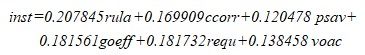
INST is a composite index of governance and was computed from six dimensions of governance using Principal Component Analysis, a statistical technique used for data reduction, and based on the six aggregate dimensions of governance- Rule of Law (rula), Control of Corruption (ccorr), Political Stability (psav), Government Effectiveness (goeff), Regulatory Quality (requ), Voice and Accountability (voac). The indices for the dimension were taken from World Bank (31). The dimension indices range from –2.5 (the lowest performance) to 2.5 (the higher performance) Composite Index was computed as
[Due to technical limitations, this equation is only available as a download in the supplemental files section.]
Where the coefficient of each variable were obtained from the square of principal component that add up to unity.
Yield was taken from the World Bank and the source defined it as kilograms per hectare, but here converted to quintal per hectare, of harvested land, includes wheat, rice, maize, barley, oats, rye, millet, sorghum, buckwheat, and mixed grains. Production data on cereals relate to crops harvested for dry grain only. The study used cross-section and annual time series data from 2000 to 2017 for 34 low income countries (29).
Estimation methods
To estimate the short run health function given in equation [8] econometric methods were applied to panel data. The method considers multiple cross-section measures over multiple time series data together to get more reliable parameter estimates than what cross-section or time series approach alone cannot address. Following the specification given in equation the marginal effect of HDA, GDPP and YIELD were assumed to vary inversely with the previous level of IMR and hence log transformation of these variables were taken for estimation. On the other hand, the marginal effects of HC and INST were assumed to have exponential relation with the previous level of IMR as these inputs are non-subtractable in their very nature. Hence their exponential transformation was used in the estimation process. The marginal effect of AFERT and EDEP were assumed to be constant since they are indices or ratios. Hence they were entered to the function without transformation.
Under the assumption of equation [8], the econometric specification that relates health status to a vector of explanatory variables is given as
[Due to technical limitations, this equation is only available as a download in the supplemental files section.]
where W(i, t) is Infant mortality rate, W(i, t-1) one period lagged infant mortality, 1nW1(i, t) is log-health development assistance for health, 1nW2(i, t) is log-GDP per capita, 1nW3(i, t) is log yield expW4(i, t) is exponential of human capital index, expW5(i, t) is exponential of governance index, expW6(i, t) is adolescent fertility rate, expW7(i, t) is elderly dependency rate, in country i at time t for i = 1,2,...34 (number of countries), t = 1,2,..17 (number of time units), 𝜀(i,t) is error term with the property E[e(i,t)] = 0 and var[e(i,t)] = (𝜎𝜀)2; 𝜇0 is constant term; 𝜇1(i) and 𝜇2(t) are country and time specific effects respectively.
To estimate equation [9] the first difference generalized method of moments (GMM) developed by Arellano and Bond (23) is suitable. Furthermore, based on the nature of the error terms, system GMM developed by Blundel and Bond depending is recommended (24). However, in the cases of a weak instrument problem in a dynamic panel data model like equation [9], first differenced GMM estimator have been found to have a poor precision (25). Therefore, system GMM estimator is recommended to provide better accurate estimate in the current IMR equation (5, 8, 26, and 27). However, for comparison purpose, estimation results from both estimators will be considered in the current study. At the same time, the conventionally derived variance estimator for GMM estimation is employed for standard error vce (gmm).
To deal with omitted variables, it is assumed that the omitted variables follow auto regressive of order one, which is equivalent to assuming that they follow first order differential equations, whose solution will be function of time. On this ground instead of just assuming the variables away, log-time is used as a control variable representing all omitted variables in both short run and long run health equations.