2.1. Parametric Coefficient. Presence of Atypical Samples
Regarding the samples, no outlier (consistently out of the limits defined by the 95% ellipses or clustered at a high dissimilarity (HCA)) was observed with PCA, HCA and PLS plots in the log-transformed data, but 6 samples were dissimilar (regularly out of or close to the limits) from the group they belong to: CRC18, HC23, R-CRC38, R-CRC46, R-HC56 and R-HC58 (see SI S-1A). In the raw data, we detected two outliers: CRC18 and HC37, and 4 dissimilar points: CRC17, R-CRC38, R-HC56 and R-HC65. Overall, the best homogenization of the samples in each subgroup was obtained with the log transformation, particularly when looking at the HCA plots.
Based on the robust z-scores and the relative ranks, one outlier: HC37, and 4 dissimilar points: CRC14, CRC18, HC32 and R-CRC38 were detected in the log-transformed data (SI S-1B). Similarly, 6 outliers were observed in the raw data: CRC18, HC37, R-CRC38, RCRC-39, R-CRC40 and R-HC57, along with 4 dissimilar points: CRC9, CRC17, R-HC55 and R-HC56. Overall, CRC 18 and R-CRC38 were consistently found as dissimilar points in the log-transformed data while CRC18 and HC37 were consensus outliers and CRC 17, R-CRC38 and R-HC56 were found consensus dissimilar points in the raw data. Again, as expected, the log transformation made the data more gaussian and less sensitive to the atypical samples. And this procedure showed efficient to highlight the main atypical samples.
2.2. Parametric Coefficient. Presence of Atypical Values
Many atypical values were observed in all four groups. Indeed, in the 29 selected correlations, we found 36 variables that had at least one outlier and 45 variables that had at least one outlier or one dissimilar value in the raw data, for a total of 55 outliers and 69 dissimilar values. After the log transformation, 19 variables had a least one outlier and 42 had at least one outlier or one dissimilar value, for a total of 24 outliers and 53 dissimilar values. Globally, for each type of data, 27 correlations had at least one outlier or one dissimilar value while 25 (raw data) and 14 (log-transformed data) had at least one outlier. This is likely because the 29 correlations were selected precisely for their differences of values between the coefficients, which is probably due to the presence of outliers. In addition, we observed that the atypical values in the raw and log-transformed data were often high and low ones, respectively (SI S-2A). This is likely due to the application of the log transformation, which reduces the right skewness of a distribution by moving it globally to the left, to (almost) symmetrical data. As for the atypical samples, we also confirmed on our specific data set that the log-transformed data were less prone to atypical values, especially to outliers. From a methodological point of view, looking at the detection methods, in almost half the cases, univariate (boxplots and Grubbs and Dixon tests) and multivariate (2D scatterplots) tools were in agreement. However, in agreement with previous observations [25], bivariate visualization was found useful to take into account the alignment of a value with the other points of a specific correlation as well as to evaluate properly the reality of the correlation [24, 26] (SI S-2B). Indeed, the alignment was found responsible for the different status (normal value, dissimilar one or outlier) of a single value according to the correlation involved. As the Dixon test is limited to the detection of one outlier, it logically underestimated the presence of outliers. Therefore, it is overall recommended to use Grubbs test and boxplots, along with scatterplots that allow to visualize the correlations by considering both variables simultaneously, and to pay particular attention to the non-aligned values. Finaly, the percentages of outliers and dissimilar values in the selected correlations designated the CRC sample 18 as an outlier and the HC sample 19 as a dissimilar sample in the raw data, with respectively 38 and 12% of outlier values and 45 and 33% of dissimilar values. In the log-transformed data, they highlighted the CRC sample 18 as a dissimilar sample with 21% and 29% of outlier and dissimilar values.
2.3. Effect of Atypical Samples and Values on r and Z
Combining the results above, it was found that the samples CRC18 and HC37 were potential outliers in the raw data while CRC17, R-CRC38 and R-HC56 were dissimilar samples. In the log-transformed data, CRC18 and R-CRC38 were dissimilar samples. The effect of those atypical samples was assessed by removing them, which is equivalent to a skipped-correlation coefficient [25, 27], and by comparing the values of r and Z (ZCRC and ZR-CRC) with and without them [26]. Other options exist that were tested elsewhere and found less powerful and less efficient [25], particularly with bivariate outliers, such as the winsorizing of the data [28] or the use of alternative coefficients such as Tukey’s biweight [29] or a percentage bend Pearson coefficient [30]. As expected, the dissimilar samples were less influential than the outliers, especially for Z where the effect of atypical samples in two subgroups could combine (Tables 1 and 2). In addition, the dissimilar samples in the log-transformed data (CRC 18) and in the raw data (R-CRC 1) produced similar absolute and relative differences, for both r and Z.
Table 1
Effect of the atypical samples on Pearson’s r.
|
r
|
Mean
|
Median
|
|
Absolute
|
%
|
Absolute
|
%
|
|
CRC
|
Raw
|
1 Outlier
|
0.21
|
221
|
0.15
|
58
|
|
HC
|
Raw
|
1 Outlier
|
0.16
|
313
|
0.08
|
41
|
|
CRC
|
Raw
|
1 Dissimilar
|
0.07
|
95
|
0.03
|
17
|
|
R-CRC
|
Raw
|
1 Dissimilar
|
0.13
|
197
|
0.06
|
28
|
|
R-HC
|
Raw
|
1 Dissimilar
|
0.04
|
64
|
0.02
|
10
|
|
CRC
|
Log
|
1 Dissimilar
|
0.09
|
158
|
0.06
|
23
|
|
R-CRC
|
Log
|
1 Dissimilar
|
0.09
|
169
|
0.06
|
22
|
Mean and median absolute and relative (in percentage of the correlation values with the outliers) differences of Pearson’s correlation coefficients r in the four subgroups of samples, for all the 5151 correlations in the data set, when removing the atypical samples.
Table 2
Effect of the atypical samples on the differential correlation coefficient ZCRC and ZR-CRC.
|
Z
|
Mean
|
Median
|
|
Absolute
|
%
|
Absolute
|
%
|
|
CRC / HC Raw – 2 Outliers
|
0.96
|
332
|
0.74
|
95
|
|
CRC / HC Raw – 1 Dissimilar
|
0.22
|
102
|
0.10
|
16
|
|
R-CRC / R-HC Raw – 2 Dissimilar
|
0.44
|
249
|
0.23
|
37
|
|
CRC / HC Log – 1 Dissimilar
|
0.28
|
138
|
0.17
|
29
|
|
R-CRC / R-HC Log – 1 Dissimilar
|
0.25
|
132
|
0.17
|
25
|
Mean and median absolute and relative (in percentage of the correlation values with the outliers) differences of the differential ZCRC and ZR-CRC, for all 5151 correlations in the data set, when removing the atypical samples.
The atypical values also had a clear effect on Pearson’s r and on the differential Z, especially with the raw data (Table 3). Again, and as expected, the raw data were more sensitive to the presence of atypical values than the log-transformed ones [26], but the two suffered from this phenomenon. Therefore, the log transformation revealed efficient but not sufficient to make the GC×GC-TOF-MS data fully gaussian.
This was observed visually on the scatterplots where the deviant values biased the linear regressions and the corresponding angles between them [24, 26] (SI S-3A). When considering the angles, scaling the data prior to the calculation was reported to be of importance to perform a relevant analysis and to avoid misinterpretations [16]. Four types of scaling were tested, consisting in the multiplication of the slopes of the linear regressions by the ratio of the means, the medians, the maxima or the ranges of values of the subgroups considered (CRC and HC or R-CRC and R-HC). Logically since the correlations values depend on the range of observations [31], we found that the range method was the most consistent with the associations observed in the scatterplots as well as with the angles calculated on the ranks, taken as the reference since they measure the metabolites on the same scale and thus do not require any change (SI S-3B). The results obtained confirmed what was seen with the numerical calculations since with the raw data, even the dissimilar values were influential, while with the log-transformed data, only the clear outliers represented an issue (SI S-3C). Overall, and to conclude on this section, when using Pearson’s r on GC×GC-TOF-MS, we found appropriate to use the log-transformed data along with a proper, uni- and multivariate outlier detection strategy, that includes a visual control through 2D graphical representations [26], in order to look for the presence of atypical samples and values. In our view, the same procedure could be applied to biomarker research as well, particularly if non-parametric statistical methods are not included in the biomarker selection process.
|
%
|
r
|
Z
|
Table 3
Effect of the atypical values on Pearson’s r and on the differential ZCRC and ZR-CRC.
|
Absolute
|
r
|
Z
|
|
Raw
|
Outliers
|
All atypical
|
Outliers
|
All atypical
|
|
Mean
|
0.21
|
0.28
|
1.34
|
1.62
|
|
Median
|
0.12
|
0.21
|
0.63
|
0.95
|
|
Log
|
Outliers
|
All atypical
|
Outliers
|
All atypical
|
|
Mean
|
0.06
|
0.13
|
0.40
|
0.74
|
|
Median
|
0.00
|
0.08
|
0.00
|
0.68
|
|
Raw
|
Outliers
|
All atypical
|
Outliers
|
All atypical
|
|
Mean
|
99
|
136
|
98
|
124
|
|
Median
|
31
|
64
|
60
|
74
|
|
Log
|
Outliers
|
All atypical
|
Outliers
|
All atypical
|
|
Mean
|
18
|
44
|
20
|
44
|
|
Median
|
0
|
17
|
0
|
29
|
Mean and median absolute (above) and relative (in percentage of the (variation of) correlation values with the outliers, below) differences between the correlation coefficients r and their variations ZCRC and ZR-CRC with and without the outliers or all atypical values, for all 5151 correlations.
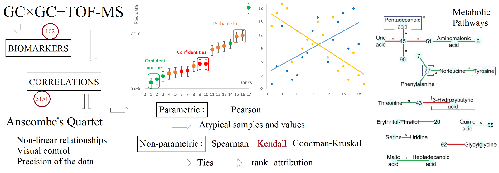
2.4. Non-parametric Coefficients. Presence of Ties through Analytical Precision
To begin with, thresholds were defined to distinguish between ties from non-ties. The three ways selected to assess the presence of ties agreed that a distance under 10% of the combined RSD of two consecutive values, which corresponds to a very small effect size (< 0.2), a t-value < 0.6 and a corresponding probability of rejecting the tie hypothesis (p-value) of less than 70%, could be seen as a confident tie (Table 4). On the contrary, a distance over 40% of the combined RSD, which corresponds to a large effect size (> 0.8), a t-value > 2.4 and a corresponding p-value > 99%, was a confident non-tie. In between, the decision was less clear but it appeared that under 25% of the RSD, equivalent to a medium effect size (0.5), a t-value of 1.5 and a p-value of 90%, the points were probably tied, while over those values they were likely to be not. The thresholds were confirmed visually through scatterplots of the raw data against their respective ranks, constructed for 8 metabolites manually selected as representatively distributed over the data set. To take the uncertainty of measure into account, error bars were drawn that were equal to combined the RSD in the QC samples (Fig. 1). In addition, the signal axis was log-transformed when the data range exceeded 10, which was often the case. As observed by Anscombe [24], this allowed the lowest signals and their error bars to be visible in comparison to the highest ones. Overall, the thresholds made sense visually for our specific data set but were also consistent with the more standard notions of effect size, t-values and p-values, which tends to show that the procedure and the criteria are generalizable to other studies, while the thresholds values would likely have to be adapted, particularly as a function of the sample size and the dynamic range of the detector (SI S-4).
Table 4
Defined thresholds for confident and probable ties and non-ties.
| |
t-value
|
p-value* (%)
|
Hedges’s g
|
RSD (%)
|
|
Confident tie
|
0.60
|
70
|
0.20
|
10
|
|
Probable (non-) tie
|
1.50
|
92
|
0.50
|
25
|
|
Confident non-tie
|
2.40
|
99
|
0.80
|
40
|
| * p-values for sample sizes 17 ≤ n ≤ 19. |
The application of the thresholds to the entire data set showed numerous ties and groups of ties (Table 5), with frequent ‘chains’ of ties difficult to interpret. The resultant number of points left to calculate the correlations was reduced by 30% and more than 50% with the confident and probable ties, respectively. As a result, the precision of the data appeared to be low in comparison to the distances between consecutive values to get confident rank attributions. Despite the care taken in the measurements and the partial correction of the peak volumes for the analytical variation measured in the QC samples through a locally estimated scatterplot smoothing (LOESS) procedure [32]. This led to what we regard as an excessive attribution of the ranks that could impair the efficiency of the non-parametric correlation coefficients if this issue is not raised, which, again, depends on the specific case at hand through both the sample size and the dynamic range of the analytical method employed. On the other hand, the frequency of such a case in the GC×GC-TOFMS data set analyzed here, and the consecutive reduction of the number of points left to evaluate the correlations could also be a problem, which tends to favour the consideration of the confident ties against the probable ones.
The effect of the ties on the correlations was moderate in absolute values (0.03 mean and median variations of the coefficients due to the confident ties, 0.05–0.1 for the probable ones), especially in comparison to the changes induced in Pearson’s r by the atypical values, but it was important in relative terms. Indeed, the median and mean variations were respectively around 10 and 40% when considering the confident ties and around 30 and 120% when considering the probable ones. The differential correlation coefficient ZCRC was influenced by the ties in a similar manner, with median and mean variations both around 0.05–0.1 in absolute values and respectively around 20 and 80% in relative terms for the confident ties. For the probable ones, the median and mean variations were both around 0.3 and 0.7 in absolute values, representing around 40 and 200% median and mean relative variations. Logically, the significant variations of correlations were also influenced by the ties: their number remained the same (but their identity changed) in the case of Spearman and it was increased with Goodman-Kruskal as well as with Kendall, but in a lesser extent. Detailed results for this entire section are given in SI S-5. The higher inflation of Goodman-Kruskal due to the ties could be explained by the fact that it explicitly takes them into account, through an adjustment of the sample size, while Kendall’s tau leaves them aside from the correlation calculation. However, it is also argued that this phenomenon could be due to its implicit directional nature that automatically uses the narrower variable as the independent one [33, 34]. The detailed visual evaluation of the 8 selected correlations confirmed the effect of the ties but it was found somewhat limited, particularly on the regressions and with the confident ties, as illustrated in Fig. 2.
Table 5
Ties, groups of ties and numbers of points left in the data set.
|
Number
|
Groups of ties
|
Ties
|
Points left
|
|
Confident
|
Probable
|
Confident
|
Probable
|
Confident
|
Probable
|
|
Mean
|
3.5
|
3.8
|
9.0
|
14.0
|
13.0
|
8.3
|
|
Median
|
3
|
4
|
9
|
14
|
13
|
9
|
|
%
|
Confident
|
Probable
|
Confident
|
Probable
|
Confident
|
Probable
|
|
Mean
|
19
|
21
|
49
|
75
|
70
|
45
|
|
Median
|
16
|
22
|
49
|
76
|
70
|
49
|
Mean and median aggregated numbers (above) and percentages (below) of groups of ties, ties and numbers of points left when considering the confident and probable ties.
Regarding the coefficients, it comes from our results, detailed in SI S5 and S-6, that with no ties or the only confident ties, Spearman’s rho was the most different coefficient of the three (the highest, with a mean rank of 1.1, in Table S17, panels A and C ; see also the left part of Table S11 for the absolute values). However, when the probable ties were taken into account, Goodman-Kruskal’s gamma caught up and Kendall’s tau became the coefficient with the most different values (with the lowest mean rank of 2.9, panel C of Table S17). After transforming Kendall’s tau and Goodman-Kruskal’s gamma to be directly comparable to Pearson’s r and Spearman’s rho [35] (right part of Table S11 and panels B and D of Table S17), they were much closer to Spearman at first (no tie) and then their inflation due to the ties, in addition to separate them from Spearman as well as from each other, made them the highest coefficients. Again, this affected particularly Goodman-Kruskal’s gamma that became the most different coefficient (mean ranks of 1.1 and 1.0 with the confident and probable ties, panel D of Table S17). Those observations were confirmed by the differential correlation coefficient ZCRC (Tables S14 for the absolute values and S18 for the differences between coefficients). Overall, Goodman-Kruskal was found the most liberal coefficient, and Spearman the most conservative, both by quite far, especially with the ties. Globally, the mean and median correlation coefficients r and differential ZCRC were relatively low, with respective values of 0.2–0.3 (up to 0.4 for Goodman-Kruskal after transformation and the consideration of the ties, Table S11) and 0.7 (up to 1 and more for Goodman-Kruskal when considering the ties, Table S14). The 75th percentiles were moderate, respectively around 0.4 (up to 0.6 for G-K) and a bit more than 1 (up to 1.8 for G- K). While the comparison between the non-parametric coefficients will be continued in the next section, it already comes from this investigation of the ties and their effects that, in order to take them into account without risking to artificially change the results, it seems a good compromise to calculate those coefficients with only the confident ties. To conclude on this section, when using a non-parametric correlation coefficient, it appears important to consider the presence of possible ties that could bias the results. To do so, the proposed strategy based on the definition and application of specific thresholds for three parameters able to highlight such ties, and the evaluation of their effects on the data and the various coefficients worked well on our GC×GC-TOF-MS data set and should be generalizable, given that the results are properly adjusted to the specific case considered.
2.5. Determination of the appropriate coefficient
To find the appropriate coefficient to perform the correlation analysis, here on our untargeted metabolomics GC×GC-TOFMS data set, the methodology consisted in comparing Pearson’s r calculated on the log-transformed data, without the outlier samples and values previously determined, to the non-parametric coefficients applied with the consideration of the confident ties. We first assessed the aggregated (5151 correlations) absolute values for both the correlation coefficients and their differential ZCRC. The first ones and their respective ranks were quite similar for the four coefficients. Spearman’s rho and Goodman-Kruskal’s gamma were the most different coefficients with respectively the lowest and highest values (0.28 and 0.34, mean ranks of 1.5 and 3.2; Table 6). The aggregated absolute differences between the coefficients, however, showed that the parametric one, Pearson’s r, was the most different. Thus, the effect of the confident ties to separate the non-parametric measures from each other was not sufficient in comparison to the difference between parametric and non-parametric coefficients. Kendall’s tau, despite being very close to Goodman-Kruskal’s gamma, was the most central coefficient, with no maximum and only 11% of minimum values.
Table 6
Comparison of the correlation coefficients.
|
Distribution
|
P
|
G-K
|
K
|
Sp
|
|
|
|
0,25
|
0.13
|
0.15
|
0.14
|
0.12
|
|
|
|
Mean
|
0.30
|
0.34
|
0.32
|
0.28
|
|
|
|
Median
|
0.27
|
0.31
|
0.29
|
0.25
|
|
|
|
0,75
|
0.44
|
0.50
|
0.47
|
0.42
|
|
|
|
Max
|
1.00
|
1.00
|
0.99
|
0.98
|
|
|
|
Mean Rank
|
2.7
|
1.5
|
2.6
|
3.2
|
|
|
|
Median Rank
|
3
|
1
|
2
|
3
|
|
|
|
% of Max
|
35
|
60
|
0
|
5
|
|
|
|
% of Min
|
43
|
0
|
11
|
45
|
|
|
|
Distribution
|
P / G-K
|
P / K
|
P / Sp
|
G-K / K
|
G-K / Sp
|
K / Sp
|
|
0,25
|
0.04
|
0.03
|
0.03
|
0.01
|
0.02
|
0.02
|
|
Mean
|
0.10
|
0.09
|
0.08
|
0.02
|
0.06
|
0.04
|
|
Median
|
0.08
|
0.07
|
0.06
|
0.01
|
0.05
|
0.04
|
|
0,75
|
0.14
|
0.13
|
0.12
|
0.02
|
0.08
|
0.06
|
|
Max
|
0.86
|
0.87
|
0.91
|
0.12
|
0.25
|
0.18
|
Aggregated absolute values, ranks and absolute differences between the correlation coefficients, for all 5151 correlations. Goodman-Kruskal’s gamma (G-K) and Kendall’s tau (K) were transformed to be directly comparable to Pearson’s r (P) and Spearman’s rho (Sp) [35].
Those observations were confirmed, and even amplified, in the aggregated differential correlations ZCRC, particularly regarding the difference between Pearson’s r and the non-parametric coefficients (Table 7). The number of significant variations of correlations led to the same conclusions, whatever the threshold used, with a ranking of the coefficients from the more liberal to the more conservative: Goodman-Kruskal’s gamma > Kendall’s tau > Pearson’s r > Spearman’s rho (Table 8). Regarding the thresholds for significance, the 0.05 and 0.01 p-values, used in the absence of appropriate direct thresholds for the correlation coefficients [36], led to dozens and even hundreds (with 0.05 and/or ties) of significant results. However, when Bonferroni and Benjamini-Yekutieli corrections for multiple testing were introduced (0.05 p-value threshold) [25, 37], very few results were left for further exploitation (Table 8). Given the exploratory nature of the procedure, and the fact that the true significance can only be achieved through replication [22, 38], we found most appropriate to compromise between the quality (necessary with low sample sizes [16]) and the quantity of the results [25] through an uncorrected p-value threshold of 0.001.
Table 7
Comparison of the differential correlation coefficients ZCRC.
|
Distribution
|
P
|
G-K
|
K
|
Sp
|
|
|
0,25
|
0.31
|
0.36
|
0.34
|
0.29
|
|
|
Mean
|
0.80
|
0.92
|
0.87
|
0.76
|
|
|
Median
|
0.66
|
0.77
|
0.73
|
0.64
|
|
|
0,75
|
1.16
|
1.33
|
1.26
|
1.09
|
|
|
Max
|
8.64
|
5.13
|
4.77
|
4.18
|
|
|
Distribution of the diff.
|
P
|
G-K
|
K
|
Sp
|
|
|
Mean Rank
|
2.7
|
2.5
|
2.4
|
2.4
|
|
|
Median Rank
|
3
|
3
|
2
|
2
|
|
|
Number of Max
|
1836
|
1547
|
394
|
1374
|
|
|
% of Max
|
36
|
30
|
8
|
27
|
|
|
Number of Min
|
2559
|
1436
|
256
|
900
|
|
|
% of Min
|
50
|
28
|
5
|
17
|
|
|
Distribution of the diff.
|
P / G-K
|
P / K
|
P / Sp
|
G-K / K
|
G-K / Sp
|
K / Sp
|
|
0,25
|
0.19
|
0.17
|
0.15
|
0.02
|
0.08
|
0.06
|
|
Mean
|
0.48
|
0.45
|
0.41
|
0.06
|
0.21
|
0.16
|
|
Median
|
0.39
|
0.36
|
0.33
|
0.04
|
0.17
|
0.13
|
|
0,75
|
0.68
|
0.64
|
0.57
|
0.08
|
0.29
|
0.23
|
|
Max
|
10.63
|
10.42
|
10.16
|
1.05
|
1.55
|
0.86
|
Aggregated absolute values, ranks and absolute differences between the differential correlation coefficients, for all 5151 correlations. Pearson’s r (P), Goodman-Kruskal’s gamma (G-K), Kendall’s tau (K) and Spearman’s rho (Sp).
Table 8
Comparison of the significant differential correlation coefficients ZCRC.
|
Threshold Uncorrected α
|
P
|
G-K
|
K
|
Sp
|
|
5.10− 2
|
284
|
492
|
397
|
221
|
|
10− 2
|
59
|
139
|
104
|
47
|
|
10− 3
|
9
|
38
|
17
|
5
|
|
10− 4
|
1
|
7
|
3
|
1
|
|
Bonferroni
|
1
|
3
|
1
|
0
|
|
BY
|
1
|
1
|
0
|
0
|
Numbers of significant variations of differential correlations coefficients Z between CRC and R-CRC samples, depending on the threshold considered, for all 5151 correlations in the data set. Pearson’s r (P), Goodman-Kruskal’s gamma (G-K), Kendall’s tau (K) and Spearman’s rho (Sp).
Given the recognized capacity of non-parametric correlation coefficients to be more robust to atypical observations (and to provide higher statistical power in their presence [39, 40]), to non-linearity and to non-normal, sparse or small data sets [34], they were expected to give a more accurate assessment of the differential correlations.
This was confirmed with the 29 selected correlations, through their numerical comparison and their visual control. It came out that all coefficients, used taking into account the outliers or the ties, gave similar results -with Pearson’s r confirmed as the most different (Fig. 3)- and seemed to correctly represent numerically the visual distributions and correlations. However, Goodman-Kruskal’s gamma tended to inflate a bit the correlations, on the contrary to Pearson’s r and Spearman’s rho who appeared sometimes to underestimate them (Table 9). Based on those observations, as well as on the previous analysis conducted on all correlations where it was found liberal but not as much as Goodman-Kruskal’s gamma, Kendall’s tau seemed the method of choice to perform an untargeted exploratory correlation study on our GC×GC-TOF MS metabolomics data. This is in agreement with the usual preference for robust algorithms in the case of atypical data, particularly with small sample sizes and unknown distributions [21, 36, 38, 41, 42]. However, this is in disagreement with the observation that, because of the way it handles them, Goodman-Kruskal’s gamma is generally preferred to Spearman or Kendall for data sets with many tied ranks [34]. This is possibly because we decided to use only the confident ties in the calculation of the correlations. In addition to the strategy that consisted in comparing the coefficients in multiple ways (aggregated values, significant results and representative cases) and revealed appropriate, the scatterplots were found very useful from a methodological point of view, confirming previous recommendations [24, 37], despite the small data sizes available leading to incomplete distributions. The use of regressions helped a lot to determine the tendencies in the data (SI S-7). Especially with moderate correlations (between 0.3 and 0.6), of which the significance was more difficult to evaluate, as well as when comparing correlations with ranges and scales that differed between the subgroups studied. Most frequently, we observed quite clear linear behaviours that were well modeled by linear regressions, which made the polynomial ones superfluous. However, the polynomial approximation, limited to the second order to avoid overfitting, could be compared to the linear regression to inform, through its curvature, about the linearity of the data. It was also able to model alternatives trends present in the subgroups of the data, again through its curvature as well as through the length of the curve on each side of it. In addition to the log-transformed data used in the calculations, the graphs included the raw data for comparison purpose. The main observation was a logical increase in linearity of the distributions through the reduction of the distances between the points.
Table 9
Differential correlations ZCRC of the 29 selected correlations for the four coefficients tested.
|
Variable
ID number
|
P
|
G-K
|
K
|
Sp
|
|
1
|
10
|
-2.0
|
-2.6
|
-2.5
|
-2.4
|
|
1
|
69
|
1.7
|
2.2
|
2.0
|
1.7
|
|
5
|
68
|
2.3
|
2.8
|
2.6
|
2.3
|
|
5
|
78
|
4.5
|
5.1
|
4.8
|
4.2
|
|
6
|
25
|
2.2
|
1.8
|
1.7
|
1.4
|
|
7
|
48
|
0.4
|
0.7
|
0.7
|
0.6
|
|
7
|
62
|
0.0
|
0.2
|
0.2
|
0.2
|
|
7
|
69
|
1.5
|
1.4
|
1.3
|
1.2
|
|
14
|
51
|
2.7
|
3.6
|
3.4
|
3.0
|
|
14
|
57
|
2.7
|
2.5
|
2.4
|
2.3
|
|
14
|
85
|
2.0
|
2.8
|
2.7
|
2.5
|
|
18
|
77
|
3.1
|
3.1
|
3.0
|
2.9
|
|
19
|
77
|
1.8
|
2.5
|
2.4
|
2.3
|
|
20
|
22
|
-1.9
|
-2.7
|
-2.5
|
-2.5
|
|
20
|
68
|
2.3
|
2.5
|
2.4
|
2.3
|
|
22
|
74
|
2.0
|
2.3
|
2.2
|
2.0
|
|
22
|
82
|
1.0
|
2.4
|
2.2
|
1.8
|
|
25
|
77
|
1.4
|
2.3
|
2.2
|
2.0
|
|
28
|
93
|
-1.9
|
-3.2
|
-2.7
|
-2.3
|
|
29
|
98
|
1.8
|
3.0
|
2.6
|
2.3
|
|
54
|
55
|
1.7
|
3.6
|
3.3
|
3.0
|
|
58
|
90
|
-1.7
|
-3.6
|
-3.3
|
-2.8
|
|
62
|
95
|
0.8
|
0.6
|
0.6
|
0.3
|
|
76
|
96
|
2.0
|
3.0
|
2.9
|
2.5
|
|
76
|
98
|
1.8
|
2.9
|
2.7
|
2.3
|
|
77
|
101
|
2.7
|
3.3
|
3.2
|
3.0
|
|
78
|
83
|
1.3
|
2.6
|
2.4
|
2.1
|
|
88
|
96
|
0.7
|
2.4
|
2.3
|
2.1
|
|
89
|
91
|
-1.9
|
-2.0
|
-1.8
|
-1.5
|
The values which absolute difference with the nearest other coefficient is ≥ 0.5 and 1, the empirical thresholds chosen to represent the medium and large differences, are respectively in light grey and grey. Pearson’s r (P), Goodman-Kruskal’s gamma (G-K), Kendall’s tau (K) and Spearman’s rho (Sp).
2.6. Specific Significant Variations of Correlations Associated to Colorectal Cancer
Using the 0.001 p-value threshold chosen above led to the selection of 17 correlations significantly altered in the “active” state of colorectal cancer (CRC samples) in comparison to the gender and age matched healthy controls (HC samples; Table 10). Among those, 10 were found specific to the active state in comparison to the CRC samples in remission (R-CRC).
Table 10
Differential correlations Z and associated p-values for the indirect comparison between CRC and R-CRC samples
|
Variable
ID numbers
|
ZCRC
|
p-value
|
ZR−CRC
|
ZCRC/R−CRC
|
p-value
|
|
5
|
78
|
4.8
|
0.000002
|
0.7
|
4.1
|
0.00004
|
|
45
|
57
|
-4.3
|
0.00002
|
-0.5
|
-3.8
|
0.0001
|
|
77
|
98
|
4.2
|
0.00003
|
0.6
|
3.6
|
0.0003
|
|
45
|
90
|
-3.8
|
0.0001
|
-0.1
|
-3.8
|
0.0002
|
|
7
|
77
|
3.8
|
0.0002
|
0.9
|
2.9
|
0.004
|
|
20
|
95
|
3.7
|
0.0002
|
0.9
|
2.8
|
0.005
|
|
8
|
43
|
3.6
|
0.0003
|
-0.6
|
4.2
|
0.00003
|
|
44
|
92
|
-3.5
|
0.0004
|
-1.4
|
-2.1
|
0.033
|
|
3
|
43
|
-3.5
|
0.0004
|
-1.1
|
-2.4
|
0.014
|
|
14
|
51
|
3.4
|
0.0007
|
1.9
|
1.5
|
0.14
|
|
54
|
55
|
3.3
|
0.0008
|
-0.9
|
4.3
|
0.00002
|
|
45
|
70
|
-3.3
|
0.0008
|
-0.1
|
-3.2
|
0.001
|
|
6
|
14
|
3.3
|
0.0009
|
0.7
|
2.6
|
0.009
|
|
45
|
51
|
-3.3
|
0.0009
|
-0.1
|
-3.2
|
0.001
|
|
29
|
77
|
3.3
|
0.0010
|
0.6
|
2.7
|
0.008
|
|
56
|
98
|
3.3
|
0.0010
|
-1.1
|
4.4
|
0.00001
|
|
18
|
71
|
3.3
|
0.0010
|
-2.9
|
6.2
|
< 0.00001
|
The differential Z between CRC and R-CRC, ZCRC/R-CRC, is the difference between the two differential Z obtained individually against the gender and age matched healthy controls, ZCRC and ZR-CRC. In bold, the variations of correlations specific to CRC.
Using the mass spectra, the linear retention indices (LRI) and the exact mass led to the confident annotation (MSI level 2) of 15 molecules on the 25 unique ones involved in the correlations of interest (Table 11), providing 3 correlations with two annotated metabolites, 11 with one metabolite annotated and 3 with no metabolites annotated. All were found to have biological functions. Since the annotation of a correlation requires both metabolites to be annotated, the issue of identifying the metabolites of interest is even more crucial than in biomarker research [43–46] and therefore constitutes a major bottleneck. This is illustrated in the network visualization, where the two main metabolic hubs highlighted (metabolites 45 and 77 in the data set) could not be reliably annotated (Fig. 4). Therefore, there was limited interest to perform a specific network analysis [10] (such as hubs, connectivity, centrality parameters; Fig. 4).
Table 11
Annotation of the metabolites involved in the correlations of interest.
|
Data set
|
Metabolite
|
Molecular Formula
|
Match Factor
|
Probability
|
Theoretical LRI
|
Mesured LRI
|
Delta LRI
|
Exact Mass
|
Number of criteria met
|
|
3
|
3-Hydroxybutyric acid
|
C4H8O3
|
793
|
49.5
|
1167
|
1164
|
3
|
0.8
|
1.4
|
3
|
|
5
|
Serine
|
C3H7NO3
|
821
|
85.0
|
1368–1388
|
1372
|
6
|
0.5
|
0.0
|
3
|
|
8
|
Threonine
|
C4H9NO3
|
877
|
91.8
|
1375–1400
|
1399
|
12
|
0.2
|
0.3
|
3
|
|
14
|
Aminomalonic acid
|
C4H4NO4
|
819
|
96.0
|
1485
|
1484
|
1
|
0.1
|
0.0
|
3
|
|
18
|
Malic acid
|
C4H6O5
|
727
|
47.9
|
1478
|
1503
|
25
|
0.3
|
|
3
|
|
29
|
Phenylalanine
|
C9H11NO2
|
704
|
53.5
|
1636
|
1631
|
5
|
1.7
|
2.3
|
2*
|
|
44
|
Glycylglycine
|
C4H8N2O3
|
731
|
4.0
|
1818
|
1824
|
6
|
0.2
|
|
3
|
|
54
|
Quinic acid
|
C7H12O6
|
661
|
69.4
|
1851–1918
|
1897
|
13
|
0.6
|
0.7
|
3
|
|
56
|
Tyrosine
|
C9H11NO3
|
876
|
80.3
|
1959
|
1957
|
2
|
0.7
|
|
3
|
|
57
|
Pentadecanoic acid
|
C15H30O2
|
658
|
90.2
|
1950
|
1951
|
1
|
0.3
|
|
3
|
|
70
|
Uric acid
|
C5H4N4O3
|
745
|
60.7
|
2136
|
2140
|
4
|
4.0
|
4.4
|
2*
|
|
71
|
Heptadecanoic acid
|
C17H34O2
|
647
|
76.6
|
2146
|
2147
|
1
|
2.8
|
3.3
|
2*
|
|
78
|
Uridine
|
C9H12N2O6
|
771
|
89.5
|
2375
|
2381
|
6
|
0.1
|
|
3
|
|
95
|
Erythritol / Threitol
|
C4H10O4
|
810
|
43.9
|
1510
|
1525
|
15
|
0.0
|
0.4
|
3
|
|
98
|
Norleucine
|
C9H12NO2
|
791
|
11.0
|
1313
|
1312–1328
|
7
|
0.2
|
|
3
|
The annotation was made through full mass spectrum (library match and probability of correct annotation), LRIs (delta between the measured and theoretical values) and exact mass (mass error in ppm). In bold, the values that met the criteria defined. *Indicates that the exact mass criterium was made less strict, up to 5 ppm.
Most publications about the CRC molecular aspects studied the subtypes of CRC as well as the CRC-initiating or tumorigenesis cellular pathways [48–53]. However, alterations of the metabolic pathways have been observed in various matrices (serum, tissues, urine, feces and breath) that can be informatively compared to the ones observed in the study (Table 12 and in bold below). They include: cell energetic metabolism according to the Warburg effect [54] (glycolysis and TCA cycle), urea cycle, structural maintenance through glycerol and ketone bodies, oxydative stress, cytochrome P450 activity and lipids, amino acids, fatty acids, bile acids and nucleotides metabolisms [4, 14, 55–60] (including multiple potential contributions of the microbiota [51]). The metabolic pathways highlighted here suffer from two weaknesses. First, they are only very weakly enriched, except for aminoacyl-tRNA biosynthesis. Second, they are rather non-specific and seem to be only indirect consequences of colorectal cancer. However, just like the candidate biomarkers, the correlations of interest are only primary results, limited by the low sample size [61]. They require to be properly confirmed through a targeted quantitative analysis of the variations observed, followed by a proper validation conducted on an independent, larger set of patients, to see if they translate to different groups of patients with the same significant distributions. After that, further biological investigation would have to be performed, that ideally would lead to a better understanding of the metabolic effects of the disease process and its remission state detectable in serum samples. In this perspective, a powerful but complex approach would be to integrate other omics data obtained on the specific biological samples analyzed for this study.
Table 12
Metabolic pathways most altered when considering the highlighted candidate biomarkers and correlations of interest.
|
CB / Corr
|
Pathway Name
|
Match Status
|
|
CB + Corr
|
Aminoacyl-tRNA biosynthesis
|
5/48
|
|
CB
|
Alanine, aspartate and glutamate metabolism
|
3/28
|
|
CB + Corr*
|
Phenylalanine, tyrosine and tryptophan biosynthesis
|
2/4
|
|
CB + Corr*
|
Phenylalanine metabolism
|
2/10
|
|
CB + Corr*
|
Butanoate metabolism
|
2/15
|
|
CB
|
Glycolysis / Gluconeogenesis
|
2/26
|
|
CB
|
Glyoxylate and dicarboxylate metabolism
|
2/32
|
|
CB + Corr
|
Purine metabolism
|
2/65
|
CB + Corr* refers to the case where the same metabolite(s) was (were) highlighted in the biomarker research and the correlation analysis; CB + Corr means that different metabolites were highlighted in the two processes that are involved in the same pathway. The match status is the number of metabolites highlighted through the biomarker research and the correlation analysis over the total number of metabolites present in the pathway.
2.7. Limitations
Besides the annotation of the metabolites mentioned above, another recurrent limitation in metabolomics that was highlighted here is the analytical stability. Indeed, the generation of quality data requires high accuracy [10] and therefore suffers from the intrinsic noise present in high-dimensional data sets [62]. In addition to its effect on the non-parametric coefficient investigated above, it reduced the number of signals available to discover candidate biomarkers and correlations of interest. Missing values, besides the problem they can be for correlation calculation by producing incomplete profiles difficult to process (an issue that had no particular consequence in this work), are another important cause of the loss of potentially interesting signals. Here, despite the care given to the chromatography,the implementation of an external QC system, coupled to a LOESS partial correction, and the replacement of all missing values by the half of the lowest signal measured for the specific metabolite, the metabolic coverage was decreased by the selection of only the stable metabolites (RSD in the QC samples under 30% [20]) and the ones present in at least half the samples of any class.Therefore, through the various preprocessing steps (summarized in SI S-8), we went from 646 quality features in the chromatographic template to 102 variables corresponding to metabolites in the final data set, confirming a previous study performed on Crohn’s disease samples where 524 quality features became 183 high-quality metabolites. If it obviously downgrades any biomarker research where it linearly decreases the number of potential candidate biomarkers, it harms even more a correlation analysis where every additional variable can have potentially interesting links with every other and where, therefore, the number of correlations available is proportional to the number of metabolites at the power 2. However, such a selection seems necessary in order to get confident results, as it was shown how even lower analytical variations have a clear effect on the non-parametric correlation estimations. This drawback is shared by all analytical platforms, in various extents, and no single instrumentation is able to provide a complete and fully stable coverage of a complex sample. Because of the exploratory nature of the analysis, if the number of significant variations of correlations was limited with the threshold applied, it could nevertheless be sufficient to provide interesting metabolic insights and associations with colorectal cancer alterations and regulations. Because of those limitations, only a small number of annotated correlations of interest were obtained and thus a very small network. The last, but not the least, limitation of our study is the small sample size we used (17 ≤ n ≤ 19), due to clinical constraint. Among the several potential effects mentioned in SI S-9, the reduced statistical power and the inflation of the correlation values are the most dangerous for us. Here, we investigated not only correlations but also variations of correlation (ZCRC or ZR-CRC) and differences in the variations of correlation between different states of the pathology (ZCRC/R-CRC). This makes difficult to evaluate the power as well as the metabolic effect sizes of interest and their significance, particularly prior to the study. Indeed, the size of the variations of interest not only depends on the specific metabolites involved, like the simple correlations, but also on both the initial and final correlation values r, as investigated for Pearson’s r by (Bujang and Baharum, 2016) [63]. Power calculation applied to our study shows that with n ≥ 17, the minimal correlation value detectable with a power of 80% at a significance level of 0.05 is around 0.6 [64], which is already a large correlation. Regarding the variations of correlations, we observed that the significant ones always involved a low or medium correlation and a very high one (in absolute value). While the very high correlations are much likely inflated by the low sample size [65], the statistical power can nevertheless be estimated by calculating the sample size necessary to detect the low or medium values. With a significance threshold (type I error) of 0.05 the power to detect the variations of correlations significant at 0.05, 0.01, 0.001 and 0.0001 are respectively of 32, 38, 63 and 90%.