Noncontact Surface Roughness Evaluation of Milling Surface Using CNN-Deep Learning Models

Abstract

This paper presents the analysis of end milled machined surfaces backed with experimental and deep learning model investigations. The effect of process parameters like spindle speed, feed rate, depth of cut, cutting speed, and machining duration were investigated to find machined surface roughness using Taguchi orthogonal array. The experiments were conducted on Aluminum A3003, a common material widely used in industries. Following standard DOE using Taguchi orthogonal array, surface roughness was recorded for each machining experiment. Surface roughnesses for the current study were categorized into four classes viz., fine, smooth, rough, and coarse based on the roughness value R_a. Images of the machined surface were used to develop CNN models for surface roughness class prediction. The prediction accuracies of the CNN models were compared for five types of optimizers. It was found that RAdam optimizer performed better among others with the training and test accuracy of 96.30% and 92.91% respectively. The accuracy of the prediction is higher than 90% thus has the potential to substitute human quality control procedures, saving time, energy, and cost. Conversely, the developed CNN model can assist in acquiring preferred machining conditions in advance. Finally, it can eliminate the dependency on expensive surface roughness measuring devices and have enormous practical applications in quality control processes.

1. Introduction

Machine tool is a device for machining materials employing cutting, boring, grinding, shearing, etc. All machine tools have cutting tools that are used to remove the material being processed. The machining quality (precision, surface quality, chip shape & size, etc.) of the part not only depends on a machine tool, cutting tool, or cooling methods, it also depends on process parameters like spindle speed, feed rate, depth of cut, machining time, etc. and procedure variables like vibration, cutting force, cutting temperature, cutting speed, tool wear, material removal rate, etc. Other non-controllable parameters such as geometric shape and workpiece materials have an important contribution to the machining quality. The relationship between the controllable and uncontrollable factors is shown in figure 1.

The machining parameters and processes produce a surface texture, so it should be carefully chosen such that the surface finish after machining is usable and within a certain threshold. The threshold range and regulations for the surface roughness are mainly determined by the characteristics and purposes of the product. In general, higher precision manufacturing requires a narrow tolerance and strict regulations causing increased cost of manufacture and difficulty in processing large volumes. Failure to attain a certain roughness quality might necessitate additional machining or polishing processes.

The most common method of measuring the surface roughness of a machined workpiece is by employing a stylus. The stylus is largely used by quality inspectors to measure surface roughness for assessing quality, which is a slow process leading to higher labor costs. In addition, this method is difficult to automate, which not only reduces productivity but also acts as an obstacle to overall process efficiency. Further, there is a high risk for the stylus to damage the workpiece because of contact pressure. Although automated robots and contactless surface roughness measurement facilities using lasers or microscopes are readily available, these systems are complicated and expensive.

With the advent of Industry 4.0, traditional manufacturing and industrial practices are in the transformation to cope with modern smart technologies. Many precision machined parts are often produced using Computer Numeric Control (CNC) machine. Precision machined parts using CNC machines can be a complex structure, with very tight tolerance in machining accuracy as well as surface roughness. The term ‘smart’ generally means that the system is intelligent and fully integrated to work collaboratively and adjust in real-time with the demand and condition without the need for human intervention. Thus, Industry 4.0 is the trend towards automation using cyber-physical systems, the Internet of things (IoT), cloud computing, and artificial intelligence [1]. Machine learning (ML) and Deep Learning (DL) are a subset of artificial intelligence. ML and DL algorithms build a mathematical model based on ‘training data’, without being explicitly programmed to do so. The ML algorithms allow learning data patterns while DL structures algorithms in layers, which can be used to predict future results with high accuracy. 

End milling differs from other machining processes due to the type of tooling that is used for abrading a given material. Unlike cutters and drill bits, end mills have cutting teeth on the sides and end of the mill. End milling is widely used for machining surfaces and its performance is limited by dynamic properties of machine structure causing chatter occurrence. The occurrence of chatter causes poor accuracy, poor roughness, decrease tool life, and material removal rate. Shimoda and Fujimoto [2] proposed adaptive spindle speed selection methods to avoid and minimize chatter vibration.

Lee et al [3] reviewed machine health for diagnostic and prognostic of the smart factory. Several researchers have utilized various intelligent models for determining surface roughness. Lin et al. [4] used Fast-Fourier Transform-Deep Neural Networks (FFT-DNN) and one-dimensional convolutional neural network (1-D CNN) to extract raw data from machining vibration signals. They showed that LSTM based model suited well for higher R_a values while 1-D CNN showed higher prediction accuracy for lower R_a ranges. Ramkumar et al [5] used the Taguchi method for the prediction of Cubic Boron Nitride tool wear used for turning operation of AISI 440c material. Bhandari et al. [6] developed a machining chart based on the Taguchi experimental results, they called it a ‘micro-drilling burr-control chart’, a tool for the prediction and control of burrs for a large range of micro-drilling parameters. Kim et al [7] reviewed several machine learning algorithms and suggested their implication in the machining industry. Grzenda and Bustillo [8] used semi-supervised learning using unlabeled data for the improvement of roughness prediction of machining operation. In [9] Huang et al, proposed an online modeling surface roughness monitoring system to reduce the quality control and roughness measurement time by utilizing Grey theory. Pan et al. [10] discretized the surface roughness using vibration signals and deep learning. Bhandari and Park [11] developed a system based on DL for evaluating surface roughness from the distribution of shade on the surface of an object. Similarly, Patel et al. [12] presented a methodology to predict surface roughness using image processing, computer vision, and ML and compared two algorithms Bagging Tree and Stochastic Gradient Boosting.

The majority of the previous studies for predicting and evaluating the machining surface roughness are based on ordinary machining operations. On the other hand, precision-machined products are delicately processed, the machining traces on the surface of the workpiece are fine and the difference in machining traces due to surface roughness is subtle. Precision machining differs from ordinary machining operations in the machining parameters, superior controls, and machining environment. Furthermore, the characteristics of various cutting tools differ, for example cutting operation using single-point cutting tool vs. multi-point cutting tool, or stationary cutting tool vs. rotating cutting tool, etc. Therefore, the methodology of previous studies makes it difficult to predict and evaluate the surface roughness of a precision workpiece. For this reason, there is little data on the correlation between machining parameters and surface roughness for precision million operations on the 3XXX series aluminum alloy.

In this paper, we propose a contactless surface roughness evaluation system implemented using deep learning models that have the potential for industrial applications. The DL models were trained on 2000 images of four machining roughness classes. The roughness classes were based on the experiment surface roughness value (Ra) employing Taguchi design of experiments (DOE). The proposed system has the potential to be used without human intervention, eliminate surface damage, fast, and reliable which is well suited for smart factories. Furthermore, the prediction and classification performance of DL models is evaluated through the Precision and Recall curve and ROC curve, and confusion matrix in addition to the validation and test accuracy.

The layout of this paper is as follows. Section 2 describes the materials used in the experiment and the experimental environment. Section 3 describes the experiment plan and measurement methods, etc. Section 4 describes data acquisition for DL model training. Section 5 describes the DL models architecture. Section 6 describes details of DL training, performance evaluation, and analysis of DL models. Lastly, in section 7 the present work is summarized.

2. Materials And Machines

2.1 Material Properties

4 mm thick A3003 aluminum plates were used for this study. Aluminum A3003, is an alloy with good corrosion resistance and moderate strength. It is not heat treatable and develops strengthening from cold working only. The 3XXX alloy series use manganese as their primary alloying element enhancing corrosion resistance and tensile strength, improves low-cycle fatigue resistance, and contributes to uniform deformation [13]. The applications of A3003 alloy include sheet metal, chemical equipment, automotive parts, fuel tanks, etc. Table 1 lists some of the chemical, physical and mechanical properties of A3003 alloy.

Table 1: Chemical, physical and mechanical properties of A3003 alloy

2.2 End-mill

In our experiments, three-flute end-mills with fish tail-standard manufactured by Neotis Co. Ltd Korea were used for every set of experiments. The detailed specification of the end-mills is listed in Table 2. For each experiment, a new set of end-mill was used.

Table 2: Specification of the end-mill

2.3 Computer software and hardware

Image preprocessing, data analysis, and deep learning model training were performed in a dedicated workstation that runs with Ubuntu 18.04 LTS and Python 3.7. The DL models were built with TensorFlow 2.0 and Keras. TensorFlow is an end-to-end open-source platform for machine learning developed by Google that offers a variety of tools and development environments for building machine learning and deep learning models. Specifications of the computer are listed in table 3. 

Table 3: Computer specification for the deep learning training

3. Experiments

3.1 Experimental Setup

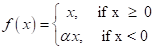
Computer Numeric Control (CNC) machines are designed to machine complex components in various industries including heavy equipment, precision machines, automotive parts, aircraft, etc. A three-axis CNC engraving machine (DAVID 3020) manufactured by DAVID Motion Technology Inc. was used for the milling experiments as shown in figure 2 (a). Single 4mm thick Al plates were used in the experiments. The lower part of the plate was supported by a force sensor which has 60mm diameter and 18.5mm height and locked by the clamp at each corner as shown in figure 2 (b). The specifications of the machine are listed in table 4.

Table 4: Specification of DAVID-3200 CNC machine

3.2 Design of Experiment (DOE) based Taguchi method

To reduce the number of experiments, a fractional matrix of experiments was used. The spindle speed (rpm), feed rate (mm/min), Depth of Cut (mm), Endmill diameter (mm), and machining time (min) were chosen as controllable parameters affecting the surface roughness of the milled part. As listed in table 5, five factors at five levels were considered to ensure that all levels and all factors are considered equally and can be evaluated independently of each other[14].

Table 5: Factors and levels of Fractional factorial design for an experiment

The effects of machining parameters on the performance characteristics can be concisely examined using the Taguchi orthogonal array (OA) design of experiments (DOE). The DOE based on the orthogonal array can be used to estimate the main effects of an experiment using only a few experimental cases. L25 (5⁵) Taguchi orthogonal array, containing the experimental parameters (viz., spindle speed, feed rate, depth of cut, end-mill diameter, and machining time) and their levels are shown in table 6. The parameter levels were selected for ease of comparison, and to find a correlation between the parameters and the surface roughness. New endmills were used for each Taguchi orthogonal matrix-based experiment.

Table 6: L25 (55) Taguchi orthogonal array used for the experiment, surface roughness values, and classes, and corresponding Vc and MRR

3.3 Surface Roughness

Surface roughness is a measure of the total spaced surface irregularities [15]. One of the common causes of surface roughness of the machined part is the occurrence of chatter. Chatter also limits the depth of cut and material removal rate of the machining process. Chatter is a self-excited machining vibration that is caused because of relative movement between the cutting tool and the workpiece causing waves on the machined surface. The productivity of machining is often limited by chatter vibration, which is an undesirable phenomenon that occurs in the machining process[16]. One of the most efficient methods to make a chatter-free machine is to make the machine, cutting tool, and workpiece as rigid as possible.

By convention 2D roughness parameters are denoted by capital R, followed by additional subscript characters as in R_a, R_q, R_z, etc. As described in ASME B46.1 [17], R_a is the arithmetic average of the roughness profile within the evaluation length. Ra values are also the most commonly used in industry because of historical reasons. The formula for calculating Ra is given in equation 1.

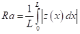
 (1)

where L is the evaluation length, Z(x) is the profile height function. 

The Mitutoyo SJ-210 surface roughness test instrument was employed to measure the surface roughness, R_a following ISO 1997 [18]. The detailed specifications of the test instrument are listed in Table 7.

Table 7: Specification of the Mitutoyo SJ-210

Three measurements were made at different locations for each milling surface. The surface measurements were performed at standard room temperature (22°C). The reported R_a values were the average of three experimental measurements. The corresponding error bars are shown in figure 3.

The surface roughness was categorized in four classes as fine (0~ 1mm), smooth (1-2mm), rough (2~4mm), and coarse (>4mm). The class number and range were determined by considering the conditions under which the experimental results are distributed in a balanced manner and the use of workpieces depending on the range of surface roughness in each class. ‘fine’ is mainly used for parts such as bearings where friction in rotating parts must be minimized. ‘smooth’ and ‘rough’ is primarily used in parts such as a high-speed rotation shaft. ‘Coarse’ is usually designated as the roughest surface roughness in parts subjected to force, vibration, and high stress.  The stylus used for measuring the surface roughness has an upper limit of R_a=10mm thus, all surface roughness over the range are listed in the fourth class, i.e., coarse.

4. Machining Surface Image Data Acquisition

The surface of the machined workpiece is shown a unique pattern of continuous ridge and valley as in figure 4. While the surface roughness of the workpiece is determined by the distance between the ridges and the valley, and the gap between the ridges and the ridges in the pattern. As mentioned previously, CNN is a highly suitable method for image classifications because of its powerful pattern recognition and feature extraction competence. Images of the machined surface were taken using the ViTiny UM12 Microscope camera magnification of 18X under fixed focus environments. The detailed specification of the ViTiny UM12 microscope camera is shown in table 8.

Table 8: Specification of the ViTiny UM12 camera

To collect images of a large number of machined surfaces, a 1-axis slide table was custom designed. The digital microscope camera was rigidly mounted above the table. The machined plate was placed on the slide table and linearly slid at 10mm/min. The machined surface was captured as color images of 640´480 pixels at 60 frames per second (FPS). A total of 167,756 images were captured with an average of 6,710 for each Taguchi experiment. The images were classified into four classes based on the surface roughness value (R_a) as listed in table 9. Corresponding experiment numbers, number of images, and other details are listed in table 9.

Table 9: Classes based on the Ra values and corresponding images

5. Deep Learning Approach

5.1 CNN Model Design

The deep neural network architecture of the CNN model presented in this study is configured such that Convolution Layer (Conv2D), Pooling Layer (MaxPooling2D), Batch Normalization, Activation Function, and Fully-connected ‘Dense’ layer sequentially repeats. Central to CNN is the convolution layer which performs convolution operation by applying the number of 2D convolution filters windows of specified height and width (kernel_size) and a stride that controls how the filter convolves across the input volume. Considering the size of the input image, the convolution kernel of size 3´3, a stride of 1, and zero-padding were used. Zero-padding fills the edge of the image with zero before convolution operation, this process maintains the size of the output and prevents vanishing of the feature on the edge of the image. 

The ‘BatchNormalization’ layers were used to standardize the data for accelerating the training and to contemplate every training data with the same scale. To progressively reduce the spatial size of the input, the ‘Maxpooling’ layer with a pool size of 2 ´ 2 and stride of 2 were used in this study. While the ‘Dense’ layer is used to feed the result of convolution layers to a Fully-Connected Neural Network and to generate a prediction. The sample code snippet is provided in table 10, and the overall model architecture is shown in figure 5.

Table 10: Code snippet of the CNN model

Gradient exploding and vanishing problems are common problems in Deep Neural Networks (DNN) that stop training in the neural network and cause performance degradation. In this study, the LeakyReLu activation function was used for effectively capturing non-linearity and solve the gradient exploding and vanishing problems. LeakyReLu introduces small negative slopes (a) to ReLU to sustain and keep the weight updates alive during the entire propagation process, this eliminates the Dying ReLu Problem. Equation 2 computes the LeakyReLu function, where a is a constant gradient (normally a=0.01).

 (2)

A comprehensive flow-chart of the study is shown in figure 6.

6. Results And Discussion

To increase computational speed under reasonable computing resources, the entire learning data were dividing into manageable batches known as minibatch. In this study, the minibatch was set to the maximum possible size (batch_size = 16) that could be handled by available computing resources. Minibatch in general improves model performance. However, the relationship between batch size and performance has not been understood well, some studies have shown that the model trained on small batch sizes showed better performance [19].

The image data-processing, CNN model architecture, training, validation, and testing codes were written in Python using TensorFlow’s implementation of the Keras high-level API. The complete code including data creation, data pre-processing, model design, and validation codes are uploaded to the Github repository and can be found at the following link https://github.com/Smart-Structure-Design-Laboratory/ENDMILL-CNN.

6.1 Train, Validation, and test data

Training and validation data were used from the original Taguchi orthogonal array experiments. The data includes the raw pixel intensities from images and their associated class labels. The first and last 10 images captured from each experiment were discarded because of unsatisfactory machining surface and image quality. The default format of the images taken by the microscope camera was the PNG format in RGB color space. The RGB images were pre-processed and converted to grayscale images, cropped to 240´240 and then saved as NumPy array for model input.

As listed in table 9, the number of images in each class is unbalanced which could cause biased results. For balancing the number of images in each class, and lowering the need for high computing resources and time, a subset of approximately 500 images in each class was randomly sampled.

The validation dataset was also created by randomly selecting images ensuring no duplicate images exist in the validation dataset and training dataset. The validation dataset had approximately 200 images for each class.

For the inference, thirteen additional experiments were performed with arbitrary machining parameters, (different from Taguchi experiments) as listed in table 11. The experimental conditions and machining surface image data acquisition methods of this additional experiment are the same as described in Section 3, however, instead of using brand new endmills, near new endmills (used for 1 to 5 minutes) were used in all the 13 additional experiments. The number of images obtained from these experiments was 7,347. The images obtained from this experiment were categorized into four classes each having 200 images.

Table 11: Additional experiment for test data images

6.2 CNN Models performance comparison

CNN is memory and computation-intensive, the number of filters on each convolution layer was limited to 64 because of workstation hardware limitation. Four hyperparameters were tuned (number of Conv2D filters, Dense layer units, learning_rate, and weight_decay) on a particular CNN model which took approximately 4 days on the workstation. Hyperparameter tuning is a technique for randomly selecting hyperparameters according to certain rules and ranges, and exploring optimal hyperparameters by training and evaluating models. It was found that the hyperparameter tuned and untuned models have slight performance differences. So, to save computation time, all the reported models in this study are hyperparameter untuned models.

Five different optimizers (SGD, RAdam, AdamW, Adamax, and rmsProp) were tested for the CNN architecture as explained above. However, because of the poor performance of rmsProp, the results of only four optimizers are reported here. The hyperparameters used for each optimizer are listed in table 12. Each model was run three times with 10, 20, and 30 epochs. In all the cases, the training and validation errors saturated in a relatively smaller number of epochs because of the large training data and a small number of classes.

Table 12: Various values of hyperparameters for optimizers

6.3 Train, validation and test accuracies

Figure 7 shows the radar plots of CNN models with four optimizers in terms of epochs, learning_rate, train accuracy, validation accuracy, and test accuracy. Note that the epochs were normalized (0-1) for clarity. All four of the presented optimizers showed outstanding accuracy of over 90% regardless of the epoch. It was seen that models trained for 10 epochs resulted in better performance, while models trained over 30 epochs experienced degraded performance due to overfitting.

Accuracy of the model varied with the selection of optimizers, superior results were received using RAdam followed by AdamW, Adamax, and SGD respectively. Here, SGD seems to have a convergence problem due to its characteristic ‘fixed’ learning rate. On the other hand, RAdam achieved more stable initial training compared to other optimizers because of the adaptive learning rate and succeeded in finding the best optimum values. AdamW showed a performance improvement with increasing epoch, although the difference was not significant, which is thought to be due to the weight decay as training progressed.

The results with the RectifiedAdam (or Radam) optimizer for 10 epochs showed the best performance with a training accuracy of 96.30% and validation accuracy of 93.31% as shown in figure 8. It can be seen that the model achieves a good fit, with train and test learning curves conversing and no sign of overfitting or underfitting. For testing the generalization of the CNN models, i.e., to check how accurately the model can predict for the new data unrelated to training data, it was evaluated by model.predict() function with the test dataset. The test accuracy was found to be 92.91%, which closely matches the validation accuracy.

Evaluating a classifier is often significantly trickier than evaluating a regressor [20]. Several model performance evaluations were performed with the best-performing CNN model. These include precision and recall curve as shown in figure 9 (a), receiver operating characteristic (ROC) curve, and confusion matrix. The precision (also called positive predictive value) and recall (also known as sensitivity) curve summarizes the trade-off between the true positive rate and the positive predictive value. The receiver operating characteristic (ROC) curve is a widely used as model’s performance evaluation metric in supervised classification problems for summarizing the trade-ff between the true positive rate and false positive rate. Figure 9 (b) shows the ROC curve, the dotted line in the figure represents the ROC curve of a purely random classifier. A well-performing classifier stays far away from the central dotted line towards the top-left corner.

In the Precision and Recall curve, the Precision rate begins to drop from the point beyond the Recall rate of 0.82. In particular, the poor performance of the rough class is noticeable, apparently due to the lack of enough training and evaluation data in the class compared to other classes. In addition, failure to extract distinct features due to the inconspicuous ridge-valley patterns between rough and smooth class might be another possible reason. Fine, smooth, and coarse class show excellent results with a precision rate of higher than 0.8 even when the recall rate approaches 1, indicating that the model is satisfactorily trained. 

The overall trend of the ROC curve matches well with the precision and recall curve. The area under the curve (AUC) is a measure of the performance of the classifier. A perfect classifier will have AUC of 1. Here, two of the classes have an AUC of 1 while the other two classes have a very high AUC value. This validates the model is generalized well. Visual observation shows that the rough class has the least AUC because of the possible causes previously explained above.

Cross-validation is often used for evaluating the model but it is not generally preferred for classification problems especially dealing with skewed datasets. For the classification task, confusion-matrix is generally considered superior to cross-validation. Figure 10 shows the confusion matrix for the model with RAdam optimizer. The most noticeable value in the confusion matrix is the predicted label for the rough class. A significant number of the coarse and smooth classes were mispredicted as rough class. This validates the Precision and Recall curves and ROC curves and reconfirms that the machined surface of the rough class is ambiguous to distinguish it from that of the smooth and coarse classes. Similarly, a small fraction of smooth classes were incorrectly predicted as fine classes, this might be because of the presence of training data with the surface roughness close to 1mm. Since 1 mm was taken as a boundary distinguishing fine class with smooth class. The classifier might have been confused with the average surface roughness value of the fine class is 0.7382mm. Other predicted classes matched well with the actual class.

From all of the model performance indicators above, it can be concluded that DL models implemented with proper architecture, and trained on relatively small surface roughness image data could have significant accuracy.

7. Conclusions

Images from DOE based on Taguchi orthogonal array were used to develop a CNN model for end-milling surface roughness class prediction. The images were acquired by capturing machined surfaces with a digital microscope. The images were converted to grayscale and cropped to 240´240, and categorized into four classes based on the surface roughness value R_a, viz., fine (0~1mm), smooth (1~2mm), rough (2~4mm), and coarse (>4mm). 500 images per class were randomly selected for training the CNN DL model. DL model training was attempted using five different optimizers. Out of the five optimizers, RAdam optimizer performed best in the given training and test data with 96.30% and 93.31% accuracy.

This study differs from other studies in that it deals with the prediction and evaluation of precision machining surface roughness on A3003 aluminum. The remarkable accuracy of the DL model even with small training data was possible because of careful design of  CNN model and selection of optimizers. The developed CNN model can assist in the accurate prediction of roughness surface, which can further assist in taking measures to suppress the chatter and avoid the unwanted roughness values in the machining process. Conversely, it can also assist in acquiring preferred machining conditions in advance. Finally, it can eliminate the dependency on expensive surface roughness measuring devices and have enormous practical applications in quality control processes.

8. Limitations and future study

Although the results from the proposed method are promising, there are some limitations with the present studies. The current study has only considered the roughness produced by endmill diameter from 1 mm to 5 mm, however, the surface roughness can be different for bigger sized endmills. The experiment for the large size endmill was limited by the CNC machine used for the experiments. Though the Taguchi orthogonal array considers the machining time, this parameter was not useful for the development of the CNN model and will be used for other analyses in the future.

In the current study, the surface roughness was classified into four classes, for the general surface quality control, it might be sufficient. However, to match ISO standards and precision manufacturing, more classes must be implemented. More insight can be received by deploying the proposed model in a real quality control environment. This will provide further insight on how to proceed with improvements to the proposed method. Future studies will focus on this aspect.

Declarations

Ethical Approval

Funding

This research is based on the partial financial support of 2020 Woosong University Academic Research Funding. 

Competing Interests

The author(s) declare no potential conflicts of interest with respect to the research, authorship, and/or publication of this article.

Availability of data and materials

The complete code including data creation, data pre-processing, model design, and validation codes are uploaded to the Github repository and can be found at the following link https://github.com/Smart-Structure-Design-Laboratory/ENDMILL-CNN.

Code availability

The complete code including data creation, data pre-processing, model design, and validation codes are uploaded to the Github repository and can be found at the following link https://github.com/Smart-Structure-Design-Laboratory/ENDMILL-CNN.

Ethics approval

Not applicable

Consent to Participate

No human participants and/or biological materials were involved in the research.

Consent for Publication

The authors consent to publication of the work presented in this manuscript. This work is not being concurrently submitted to and is not under consideration by another publisher, that the persons listed above are listed in the proper order and that no author entitled to credit has been omitted.

Authors Contributions

The first author conceived the research design, experimental setups, and partial codes of the research. 

The second author assisted in performing the experiments, gathered the experimental data, processed the data, and contributed to coding.

ORCID iD Binayak Bhandari https://orcid.org/0000-0002-4046-2379

References

1. H. Lasi, P. Fettke, H.-G. Kemper, T. Feld, and M. Hoffmann, “Industry 4.0,” Bus. Inf. Syst. Eng., vol. 6, no. 4, pp. 239–242, 2014, doi: 10.1007/s12599-014-0334-4.
2. T. Shimoda and H. Fujimoto, “Adaptive spindle-speed selection for chatter avoidance to achieve high-precision NC machining based on semi-discretization method,” in IECON 2017 - 43rd Annual Conference of the IEEE Industrial Electronics Society, 2017, pp. 6709–6714, doi: 10.1109/IECON.2017.8217172.
3. G. Y. Lee et al., “Machine health management in smart factory: A review,” J. Mech. Sci. Technol., vol. 32, no. 3, pp. 987–1009, 2018, doi: 10.1007/s12206-018-0201-1.
4. W. J. Lin, S. H. Lo, H. T. Young, and C. L. Hung, “Evaluation of deep learning neural networks for surface roughness prediction using vibration signal analysis,” Appl. Sci., vol. 9, no. 7, 2019, doi: 10.3390/app9071462.
5. V. A. Ramkumar A., Murugan M., “Assessment of Surface Roughness of Cubic Boron Nitride Influencing in Turning Process of AISI 440c Using Taguchi Method,” Taga J., vol. 14, pp. 2838–2845, 2018.
6. B. Bhandari et al., “Development of a micro-drilling burr-control chart for PCB drilling,” 2014. doi: 10.1016/j.precisioneng.2013.07.010.
7. D. H. Kim et al., “Smart Machining Process Using Machine Learning: A Review and Perspective on Machining Industry,” Int. J. Precis. Eng. Manuf. - Green Technol., vol. 5, no. 4, pp. 555–568, 2018, doi: 10.1007/s40684-018-0057-y.
8. M. Grzenda and A. Bustillo, “Semi-supervised roughness prediction with partly unlabeled vibration data streams,” J. Intell. Manuf., vol. 30, no. 2, pp. 933–945, 2019, doi: 10.1007/s10845-018-1413-z.
9. P. T. B. Huang, H. J. Zhang, and Y. C. Lin, “Development of a Grey online modeling surface roughness monitoring system in end milling operations,” J. Intell. Manuf., vol. 30, no. 4, pp. 1923–1936, 2019, doi: 10.1007/s10845-017-1361-z.
10. Y. Pan, R. Kang, Z. Dong, W. Du, S. Yin, and Y. Bao, “On-line prediction of ultrasonic elliptical vibration cutting surface roughness of tungsten heavy alloy based on deep learning,” J. Intell. Manuf., 2020, doi: 10.1007/s10845-020-01669-9.
11. B. Bhandari and G. Park, “Development of a surface roughness evaluation method from light and shade composition using deep learning,” Tranactions Smart Process. Comput., 2021.
12. D. R. Patel, H. Thakker, M. B. Kiran, and V. Vakharia, “Surface roughness prediction of machined components using gray level co-occurrence matrix and bagging tree,” FME Trans., vol. 48, no. 2, pp. 468–475, 2020, doi: 10.5937/FME2002468P.
13. S. W. Nam and D. H. Lee, “The effect of Mn on the mechanical behavior of Al alloys,” Met. Mater. Int., vol. 6, no. 1, pp. 13–16, 2000, doi: 10.1007/BF03026339.
14. “Reliability hotwire,” Reliasoft corporation, Issue 131, 2020. https://www.weibull.com/hotwire/issue131/hottopics131.htm (accessed Jan. 22, 2021).
15. J. T. Black and R. A. Kohser, DeGarmo’s Materials and Processes in Manufacturing. Wiley.
16. Y. Altintas, Manufacturing Automation: Metal Cutting Mechanics, Machine Tool Vibrations, and CNC Design, 2nd ed. Cambridge University Press, 2012.
17. Anon, Surface Texture (Surface Roughness, Waviness and Lay)., vol. 2009. 1978.
18. “ISO 4287:1997.” https://www.iso.org/standard/10132.html (accessed Jan. 20, 2021).
19. N. S. Keskar, J. Nocedal, P. T. P. Tang, D. Mudigere, and M. Smelyanskiy, “On large-batch training for deep learning: Generalization gap and sharp minima,” 5th Int. Conf. Learn. Represent. ICLR 2017 - Conf. Track Proc., pp. 1–16, 2017.
20. A. Geron, Hands-on machine-learning with scikit-learn, keras and Tensorflow-Concepts, tools, and techniques to built intelligent systems (2nd Edition. O’reilly, 2019.