Sample collection and processing
As per Veeck’s classification [6], cleavage-stage embryos that were morphologically good were defined as day 3, grade 1 or 1, seven-to-nine cell embryos. Further, according to Gardner’s score [15], morphologically good blastocysts were found to have a score of 3BB and above, and were defined as day 5 blastocysts.
The products obtained as a consequence of PCR were quantified using a Qubit fluorimeter (Invitrogen, Carlsbad, CA) and run on a bioanalyser to confirm the appearance of a single band at 350bp. Furthermore, no band was to be observed for the “kit-ome” control.
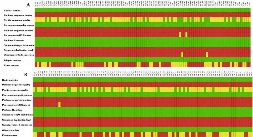
QUALITY CHECK
The supplementary figure S1 depicts the consolidated quality check result of all reads contained in the 52 samples. The different FASTQC check parameters are basic statistics, per base sequence quality, per tile sequence quality, per sequence quality score, per base sequence content, per sequence GC content, per base N content, sequence length distribution, sequence duplication level, overrepresented sequences, adapter content, k-mer content.
TAXONOMY ASSIGNMENT
RDP Database
Cervical Samples
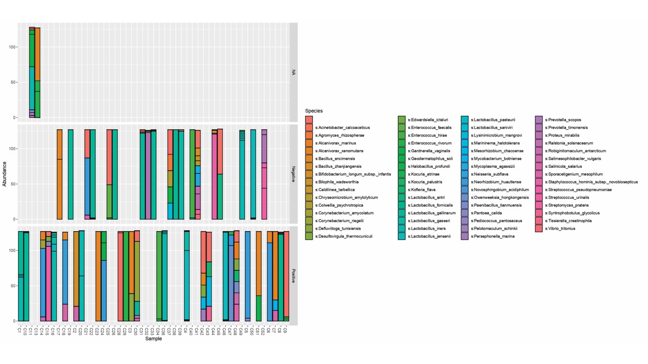
Due to a large number of species recognized, subsequent filtering was done based on abundance of the microbes within the sample. The taxa were filtered in such a way that only those OTUs were considered which represented at least 20 percent of reads in at least one sample. This filtering was done and the graph was generated at the genus level taxonomy.
Among the taxa obtained at genus level for the cervix samples, the maximum abundance is seen for Lactobacillus genus. The top genera observed were Alcanivorax, Bifidobacterium, Corynebacterium, Defluviitoga, Enterococcus, Escherichia/Shigella, Gardnerella, Geodermatophilus, Lactobacillus, Marininema, Neorhizobium, Owenweeksia, Parcubacteria_genera_incertae_sedis, Prevotella, Proteus, Staphylococcus, Streptococcus, Streptophyta. The barplot for the abundance values in cervical samples is shown in figure 1.
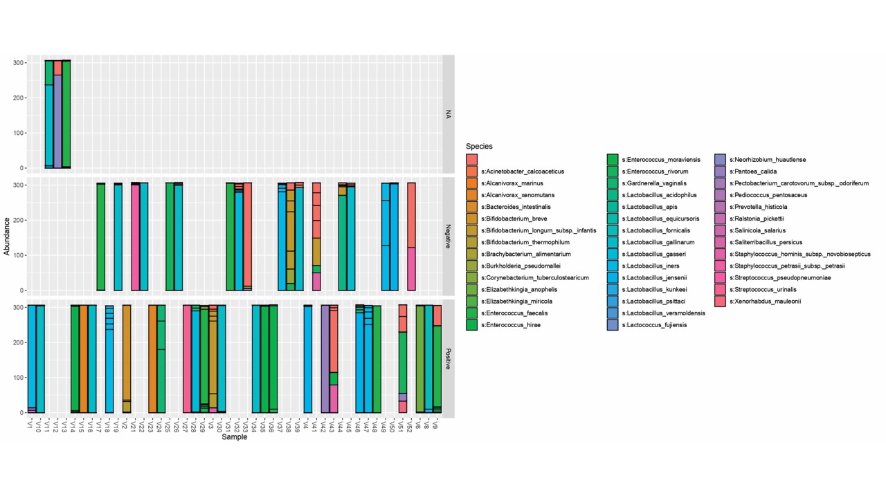
Vaginal samples
As described elsewhere, the filtering of taxa was done to obtain the genera that represent at least 20 per cent of the reads in every sample.
Here, the taxa from Negative controls were filtered off (figure 1A) and the resulting dominant taxa in vaginal samples according to RDP database are: Alcanivorax, Bifidobacterium, Elizabethkingia, Enterococcus, Escherichia/Shigella, Gardnerella, Lactobacillus, Neorhizobium, Pantoea, Staphylococcus, Streptococcus. The barplot for the abundance values in cervical samples is shown in figure 1B. The species level analysis from the RDP database for both cervix and vaginal samples is given as supplementary figure S2 and S3.
GREENGENES DATABASE
Another prominent database commonly employed in taxonomic annotation to read is the Greengenes database. It, however, reports up to the level of genus for a given sample. The graphs were generated separately for each implantation type.
The above figure 2 depicts all the possible genera obtained in each sample in comparison against Green genes database. Since a large number of organisms, filtering based on abundance was carried out and only the taxa with abundance greater than 10 per cent in a sample have been reported.
Cervix - positive implantation results
Overall, the abundant genera in cervix representing positive implantation are: Lactobacillus, Bifidobacterium, Alcanivorax, Acinetobacter, Enterobacteriaceae, Rhizobiaceae, Enterococcus, Haererehalobacter, Pelagibacteraceae, Gardnerella, Streptococcus, Ralstonia, Ureaplasma, Rhodobacteraceae. The barplot indicating the microbes in positive implantation and the abundance is shown in figure 2A.
Cervix - negative implantation results
Filtering of the genera based on its abundance in the sample (> 10%) was performed to yield the following abundant genera: Haererehalobacter, Alcanivorax, Lactobacillus, Enterococcus, Enterobacteriaceae, Staphylococcus, Proteus, Bifidobacterium, Lactococcus, Streptococcus, Haemophilus. The barplot indicating the microbes in negative implantation and the abundance is shown in figure 2B.
Vagina - Positive implantation results
The genera obtained in the vaginal samples of the infertile females are shown above. According to the filtered results, the abundant genera are: Lactobacillus, Bifidobacterium, Enterobacteriaceae, Enterococcus, Elizabethkingia, Ralstonia, Alcanivorax, Ureaplasma, Gardnerella, Streptococcus, Acinetobacter (Figure 3A).
Vagina - Negative implantation results
The result obtained for negative or unsuccessful implantation is shown above. The filtered abundant genera are: Lactobacillus, Bifidobacterium, Enterobacteriaceae, Enterococcus, Prevotella, Staphylococcus, Planococcaceae, Proteus, Alcanivorax (Figure 3B).
Microbial communities obtained having null effect on implantation success
Cervix – NA implantation results
The most abundant genera obtained in the NULL category are: Lactobacillus, Gardnerella, Ureaplasma, Haererehalobacter, Alcanivorax, Enterococcus. The barplot indicating the microbes in NA implantation and the abundance is shown in figure 4A.
Vagina – NA implantation results
The result obtained for null implantation is shown above. The filtered abundant genera are: Lactobacillus, Gardnerella, Ureaplasma, Alcanivorax, Enterococcus (Figure 4B).
Pathogenicity report of the present microbial community
The table 1 shows the list of all the genera present in all three experimental conditions (Positive, negative, not applicable) highlighting the unique and the specific genera with respect to negative outcome. The details about the pathogenicity of each of genera is given in Supplementary table S2.
Statistical Analysis
The statistical analysis of 16s rRNA data generally involves computation of alpha diversity (measure of diversity contained within a sample) and beta diversity (diversity between the samples).
Alpha Diversity
The Green genes database reports diversity till genus level of taxonomy and RDP database reports till species level of taxonomy.
Cervical Samples
The intra-sample diversity measure in the form of a violin plot is depicted in figure 5. A violin plot is a combination of a boxplot and a histogram. Here, the chosen index for representation is the Shannon’s Entropy index. Shannon Diversity index is a mathematical measure of species diversity in a community. The Shannon Diversity index also takes into account both the number of species present in a community and their relative abundance [15]. The measurement of diversity consists of two components: 1) Species Richness: these depict the number of individuals per sample: 2) Equitability Index: the different species in a community are compared in terms of evenness of their distribution; the relative abundance is measured.
A community with a high value of evenness index implies that it has the same number of individuals in different species. The number of species present in the community is said to be species richness index. For a community consisting of a single species, the least value of Shannon Index (H’) is zero. There is maximum content of information in the sample if there is high species evenness (equal number in all species) [16]. This index increases as the species richness and evenness both increases. The Shannon index also assumes that all the species are represented in the sample. Typical values of Shannon Index lie between 1.5 and 3.5 which is in confirmation to our observations of this study as shown in figure 5(Aa and Ab).
Observing the violin plots for both cervical and vaginal samples (from Green genes database), we can see that the largest value of Shannon Index is quite high compared to the limits (i.e., nearly 8 in cervix and up to 6 in vagina). In the cervix samples, it can be seen that the highest Shannon entropy is observed in the set of samples whose implantation result is positive (Figure 5Aa). The next highest Shannon Entropy is that of Negative implantation result (Figure 5Aa). The Shannon index values of vaginal samples are very low compared to the cervical samples (Figure 5Ba and Bb). The values of the index can be deduced from the inner box plot situated within the symmetrical histogram. The higher range of values in cervical samples implies higher species richness and evenness. The vaginal samples have lower species richness. But, on the other hand, if we compare the density plots surrounding the boxplot in both cervix and vagina, we can see that a majority of the values are clustered in a single place for the vaginal samples. For positive samples in the vagina, the curve almost resembles a normal distribution (Figure 5Ab and Bb). In the cervical samples however, the frequency of index values is not very high, but the range of values is quite wide (Figure 5Aa and Ba).
The plots indicate alpha diversity from the RDP database report at the species level of classification. The range of diversity depicted by the RDP database seems to be lower compared to that of the Green genes database. Additionally, the species level alpha diversity also reports overall higher diversity in the cervix samples compared to vaginal samples (Figure 5). A large proportion of the Shannon Index values are clustered within 0-1 range for the RDP database plots.
To summarize, at the genus level, Green genes database reports a high Index value depicting large species richness and evenness (with larger values in cervix compared to vagina). From the RDP database plots (at species level), it can be deduced that the diversity till species level is less. The range of alpha values are lesser compared to Green genes. This indicates that there is a wide variety of genera but a comparatively lower diversity of species among the samples.
Rarefaction Analysis
Generally, rarefaction analysis is performed to identify the species richness by the way of sampling. This is identified using the concept of rarefaction curve, which is a curve of the number of species against the number of samples. As the initial sampling is being done at the commencement of the analysis, the curve steadily rises as the most common species are rapidly being identified. However, once this is done, the curve reaches a plateau as only the rarest species are yet to be identified. The downfall of this method is that if the size of subjects being sampled keeps increasing, the number of species being identified also keeps increasing. Thus, the method of repeatedly re-sampling a given number of samples is done and the number (average) of species identified in each sample is plotted.
Three estimators are used for alpha rarefaction: chao1, observed OTUs and PD (Phylogenetic diversity) whole tree. Rarefaction is a method for creating an even number of reads for a given sample. This is crucial because during comparison of diversity, higher numbers of samples reveal rare species. Additionally, when similarities of samples are considered, there might be findings of rare species in a sample because of higher sampling depth but not in another sample. Thus, rarefaction is done to account for differences in sampling depth while comparison for similarities or differences between samples.
Rarefaction curves, however, are different from rarefaction. Rarefaction accounts for uneven/ unequal sampling size whereas rarefaction curves identify if all the diversity present in a given community is captured. The curve between the number of reads and the number of OTUs is the rarefaction curve. The flattening of the curve depicts that the sample had enough reads to identify most of the diversity contained [17].
Chao1 is a method of estimation of species richness (number of different species present in an environment) based on abundance. It is a non-parametric technique, and gives more relevance to species which have less abundance (only doubletons and singletons give the number of missing species). It assumes that rare species give most information about the number of missing species [18]. The PD whole tree is a measure of diversity which identifies, among a set of species, the degree of relatedness (in the form of a tree). It works on the basis that the diversity of a set of species is less when they are closely related and more when they are distantly related [19]. The main viewpoint of analysis of the rarefaction curve is that if the curve for any given category do not extends all the way to the right end of the X-axis, then it means that at minimum one of the samples in that category does not have enough sequences. The rarefaction analysis was conducted for both the cervical and vaginal samples (Figure 6). Since all the plots could not be displayed, alpha rarefaction curves for some of the important categories are shown.
Cervical Samples
Here, three curves have been plotted for positive result of implantation: the metadata variables considered are age (Figure 6A), assisted hatching (Figure 6B) and number of embryos transferred (Figure 6C). It can be seen that all the three curves have nearly flattened curves indicating that enough sequences per sample were present to capture the diversity. For the number of embryos transferred (Figure 6B), one curve hasn‘t completely reached the plateau.
Vaginal Samples
Amongst the vaginal samples, the alpha rarefaction curve for the following metadata categories has been included for positive result of implantation (Figure 7A), procedure opted for the assisted reproductive treatment (figure 7B) and cause of infertility and type of infertility (primary or secondary) (Figure 7C). The curve for type of procedure opted and Chao metric has not reached plateau indicating lack of sequencing depth in identification of species richness.
Beta Diversity and principal coordinate analysis
The beta diversity is calculated to identify the diversity between samples. Here, the
Weighted and Unweighted Unifrac distance measure was chosen to find if there is any
significant clustering between the samples of three outcome categories, namely Positive,
Negative and Null. Since the beta diversity measures are dissimilarity measures, higher
numbers indicate lesser similarity and more differences between the samples/ communities
under consideration.
Since the Unifrac metric is being used here as the distance measure to calculate the pairwise distances from each sample to all other samples, it results in a large distance matrix. This distance matrix is then made to undergo the ordination process, where the matrix is converted into all samples and the respective principal axes of variation in a process called ordination. Generally, three principal components are measured for easy visualization. The principal coordinate analysis (PCoA) is used to represent the ordinated matrix in the form of the first three principal axes of variation to observe any clustering based on the required outcome or metadata variable [20]. Unifrac takes into consideration the phylogenetic information for comparison of samples. The main contributing factors responsible for the variation between the microbial communities can be identified through PCoA [21]. There are two kinds of Unifrac metrics, namely weighted, also known as quantitative, which takes abundance of organisms into consideration and unweighted, which takes only its presence or absence and hence is called qualitative in nature.
Cervical Samples
Unweighted Unifrac Distance metric
The two dimensional plot of Principal Coordinate analysis performed using the unweighted Unifrac distance metric (Figure 8A). The plot is clustered by the outcome variable i.e., either Positive, Negative, Null implantation result, as it can be seen, no significant clustering can be observed between the samples across the 3 outcome variables.
Even in the weighted PCoA, the clustering is not clearly visualized among the 3 outcome variables (Figure 8B).
Vaginal Samples
Unifrac Distance metric
A similar analysis was carried out in the vaginal samples, resulting in the PCoA plots for unweighted and weighted metric (Figure 9). Here, some level of clustering can be observed from the 2-Dimensional PCoA plot in PC1vsPC2 (Figure 9A) and PC1vsPC3 plot, indicating distinct differences in the communities. The positive and negative samples are separable with a few exceptions. No significant clustering is observed for the three different outcome variables (Figure 9B).
The distance comparison using boxplot is also informative as boxplot depicts the comparison within the different levels or categories of the metadata variables. Within samples distances when compared across the 3 categories, are not very different (Figure 10). However, the positive and negative samples have similar ranges of distances and the null samples have a very small range. In the weighted UniFrac boxplot, it can be observed that though the distances are very similar indicating that the three groups are nearly identical, the range of distances is also based on the relative abundance of the community (Figure 10Aa and Ba).
Irrespective of whether the abundances are taken into consideration (weighted) or not (unweighted), the 3 communities are very similar to each other in terms of the UniFrac distance. The Positive and Null groups show significantly different means. In the unweighted boxplot, the distances seem to be higher compared to that of weighted boxplots (Figure 10Ab and Bb). The range of the distances, however, seem to be higher in the weighted box plot indicating large within sample variations due to consideration of abundance in the calculation of the distance.