To acknowledge the medical service capacity of the first batch of county-level key clinical specialties in Henan province, analyze the influencing factors, and make targeted suggestions. TOPSIS method was used to evaluate the medical service capacity comprehensively, and the influencing factors were analyzed by simple linear regression and multiple linear regression. In the multiple linear regression model, the basic conditions, including the total investment funds during the construction period, net usable area of beds and the ratio of bed to nurse, the quality of care—the compliance rate of major clinical diagnosis and pathological diagnosis, and the personnel training—the number of technical promotion trainees, of the first county-level clinical specialties, have a significant influence upon the medical service capacity; while, the actual number of beds, the ratio of doctors and nurses, the proportion of annual expert visits, the number of technical promotion training and sending of learners, percentage of drug expenditure and core journal articles have limited effect. On the basis of the ensured allocation of resources and capital investment, more attention should be paid to personnel training and appropriate technology promotion, and the medical care quality is supposed to be always insisted on, to promote the overall improvement of medical service capacity in county hospitals.
Research article
Analysis of the Influencing Factors of the Medical Service Capacity in Key Clinical Specialties at the County Level Based on TOPSIS
https://doi.org/10.21203/rs.2.20766/v2
This work is licensed under a CC BY 4.0 License
Version 2
posted
You are reading this latest preprint version
medical service capacity
influencing factor
county-level clinical key specialty
Henan province
TOPSIS
In order to further enhance the capacity of county-level hospitals, implement graded diagnosis and treatment, and achieve the goal of medical reform, the county-level clinical key specialty construction project has been implemented since 2014 in Henan province, an average of 30 specialties per year, each year for each specialty investment of 2 million yuan of construction funds. The plan is to build a number of county-level clinical advantage specialties in the province in about 5 years, aiming to promote the overall medical service capacity and medical quality management of county-level hospitals in an orderly manner, and to further play the leading role of county-level hospitals to meet the basic medical and health service needs of the local residents [1]. This paper evaluates the medical service capacity when the construction of the first batch of county-level clinical key specialties is completed, analyzes the relevant influencing factors, provides empirical basis and suggestions for the projects that are put into construction, and promotes the further improvement of the medical service capacity of county-level hospitals.
1.1 Source of Materials
The first batch of 30 county-level clinical key specialty construction projects was implemented in 2014, the construction cycle of 3 years, including 2 infectious disease department, 2 general surgery departments, 4 orthopedic departments, 5 neurology departments, 6 pediatric departments, 4 cardiovascular departments, 2 nephrology departments, 1 obstetric department, 1 gynecology department, 1 critical care unit, 1 neurosurgery and 1 oncology department. The questionnaire was designed consistent with construction objectives, the survey covered the basic conditions of specialty, medical technical team, medical service ability, medical quality and the capacity of scientific research and teaching, which were in the form of quantitative and qualitative indicators. The questionnaire was distributed among the 30 specialties, when the construction cycle is completed in 2017, with recovery rate of 100%. The data from the questionnaire survey results were used then in the TOPSIS analysis and linear correlation analysis.
1.2 Methods
According to the results of the questionnaire survey research, combining with the literature research, the index system was established, as well as the weight of each indicator. And the TOPSIS method was used to evaluate the capacity of the first batch of county-level clinical key specialty medical services in Henan Province. The medical service capacity was classified and grouped by rank and ratio (RSR). Simple linear regression analysis and multiple linear regression analysis were carried out to filter and determine the influencing factors of medical service ability by SPSS 19.0.
1.2.1 Construction of the indicator system Based on the method of literature analysis and selection, after reference to the relevant literature [2-3], the indicators related to medical service capacity in the questionnaire entered the index system, the Medical Service Ability Evaluation Index System was established, which is composed of 11 indicators that can reflect the capacity of medical services, including diagnosis and treatment ability, efficiency, innovation ability and radiation capacity, as detailed in Table 1. Among them, the high-excellent indicator is the higher the better, and the low-excellent indicator is the lower the better. The weight in the index system is based on the system of evaluation index of county-level clinical key specialty in the existing study.
Table 1 Medical Service Ability Evaluation Index System
|
Level 1 Indicator |
Level 2 Indicator |
Weight(wj) |
Code |
Character |
|
Diagnosis and Treatment Capacity |
Annual Outpatient visits |
0.032381 |
X1 |
High-excellent |
|
Annual Discharge |
0.032381 |
X2 |
High-excellent |
|
|
Percentage of Critical Cases of Difficult patients |
0.069316 |
X3 |
High-excellent |
|
|
Cure Rate for Major Diseases |
0.0843448 |
X4 |
High-excellent |
|
|
Success Rate of Difficult and Serious Rescue |
0.174113 |
X5 |
High-excellent |
|
|
Work Efficiency |
Average Inpatient Day |
0.149739 |
X6 |
Low-excellent |
|
Bed Utilization Rate |
0.045344 |
X7 |
High-excellent |
|
|
Bed Turnovers |
0.082418 |
X8 |
High-excellent |
|
|
Innovation Capability |
Number of New Technologies in the County and above |
0.054995 |
X9 |
High-excellent |
|
Annual Number of Patients Treated with The New Technology |
0.110006 |
X10 |
High-excellent |
|
|
Radiation Ability |
Percentage of Out-of-County Patients |
0.016500 |
X11 |
High-excellent |
1.2.2 Method of TOPSIS (Technique for Order Preference by Similarity to an Ideal Solution) It’s a method to find the best and worst solution sands in the space of the limited scheme of positive and negative ideal solution, and to sort and evaluate the advantages as well as disadvantages by evaluating the relative distance between the object and the optimal scheme [4]. Among the high-excellent indicators, the maximum data of the 30 evaluation objects is the optimal, while in the low excellent index, the minimum data of the 30 evaluation objects is the optimal. The data set composed of the optimal data of 11 evaluation indicators is the optimal scheme, and the worst scheme works the same way with the optimal scheme. The method has no strict restrictions on the type of data distribution, sample content, index correlation and quantity, and is often used for the overall evaluation of medical institutions, and can make full use of the original data information [5].
(1) Same trend transformation Due to the different nature of the indicators, some the higher the better, some the lower the better, it need to go through appropriate transformation so that all indexes show the same property. In this paper, the low optimal index X6 (Average Inpatient Day) was converted into high optimal index (X6’) by reciprocal method. As shown in Table 2.
Table 2 Original Medical Service Capacity Data of the First Batch of 30 County Clinical Key Specialty
|
Specialty |
X1 |
X2 |
X3 |
X4 |
X5 |
X6 |
X6‘ |
X7 |
X8 |
X9 |
X10 |
X11 |
|
A1 |
0.72 |
0.3 |
34.4 |
82.9 |
99 |
7.45 |
0.134228188 |
95 |
23.08 |
2 |
69 |
19 |
|
A2 |
0.6433 |
0.2464 |
28 |
94.1 |
86.31 |
11.55 |
0.086580087 |
97.8 |
28.5 |
5 |
324 |
20.5 |
|
A3 |
2.4158 |
0.6015 |
4.53 |
83.3 |
34.83 |
10.6 |
0.094339623 |
123 |
41 |
2 |
109 |
3.5 |
|
A4 |
0.7 |
0.85 |
29.24 |
94.76 |
81.25 |
8 |
0.125 |
109 |
5.6 |
2 |
63 |
5 |
|
A5 |
1.886 |
0.4616 |
21 |
92.9 |
78.6 |
9.8 |
0.102040816 |
97.91 |
36.45 |
2 |
23 |
12.5 |
|
A6 |
0.1527 |
0.1508 |
16.58 |
70.94 |
58.33 |
14.2 |
0.070422535 |
104.52 |
36.12 |
5 |
320 |
1 |
|
A7 |
0.1527 |
0.0803 |
45.9 |
77.9 |
79.5 |
6 |
0.166666667 |
74.3 |
47.2 |
1 |
184 |
10.1 |
|
A8 |
1.198 |
0.1471 |
36.15 |
95.4 |
92.31 |
9.2 |
0.108695652 |
86.9 |
31.74 |
1 |
119 |
6.5 |
|
A9 |
28.6857 |
3.2496 |
5.4 |
87.3 |
97 |
4.7 |
0.212765957 |
96 |
7 |
2 |
150 |
11 |
|
A10 |
3.5454 |
0.1956 |
22 |
89.2 |
81.4 |
10.2 |
0.098039216 |
97.6 |
2.6 |
1 |
447 |
1.5 |
|
A11 |
0.278 |
0.1583 |
11.99 |
88.7 |
86.42 |
16.3 |
0.061349693 |
86 |
38.7 |
6 |
372 |
16 |
|
A12 |
2.6412 |
0.6454 |
40 |
77 |
56.8 |
9 |
0.111111111 |
138 |
60 |
1 |
3141 |
15 |
|
A13 |
0.416 |
0.14 |
2.1 |
69.4 |
0 |
23.4 |
0.042735043 |
100 |
32 |
3 |
38 |
8.1 |
|
A14 |
1.3878 |
0.3773 |
16.61 |
94.28 |
91.23 |
6.8 |
0.147058824 |
11.37 |
48.46 |
1 |
1065 |
7.6 |
|
A15 |
7.8252 |
0.717 |
8.663 |
97 |
90.4 |
8.1 |
0.12345679 |
85.4 |
45.4 |
3 |
3560 |
27.78 |
|
A16 |
3.807 |
0.705 |
6.7 |
87.81 |
86.66 |
12.3 |
0.081300813 |
96.82 |
20.22 |
9 |
3069 |
5 |
|
A17 |
2.3035 |
0.2247 |
3 |
87.81 |
86.53 |
11.7 |
0.085470085 |
90 |
14 |
7 |
123 |
5 |
|
A18 |
2.1385 |
0.3429 |
26 |
87.4 |
29.85 |
8.9 |
0.112359551 |
93.2 |
30 |
5 |
3020 |
41 |
|
A19 |
1.7596 |
0.3869 |
18 |
19.57 |
90.4 |
6.9 |
0.144927536 |
118 |
4.6 |
5 |
308 |
3.7 |
|
A20 |
1.8724 |
0.2044 |
12 |
95.52 |
98.81 |
8.7 |
0.114942529 |
99 |
35.12 |
5 |
472 |
11.7 |
|
A21 |
5.6586 |
0.7128 |
1.16 |
91.88 |
99.52 |
4.7 |
0.212765957 |
89 |
59.5 |
3 |
17827 |
10.17 |
|
A22 |
4.5559 |
0.125 |
1.16 |
91.22 |
90.4 |
4.7 |
0.212765957 |
90 |
22 |
5 |
520 |
17.8 |
|
A23 |
16.6421 |
0.9112 |
53 |
83.74 |
98 |
5.5 |
0.181818182 |
94.8 |
75.9 |
3 |
1508 |
8.1 |
|
A24 |
1.8842 |
0.6771 |
3.3 |
90.41 |
70 |
7.1 |
0.14084507 |
90.4 |
46 |
1 |
33 |
10.79 |
|
A25 |
1.8842 |
0.52 |
3.53 |
84.85 |
97.66 |
7.1 |
0.14084507 |
94.8 |
36.3 |
5 |
559 |
14.4 |
|
A26 |
2 |
0.803 |
17 |
91.4 |
96.33 |
8.5 |
0.117647059 |
92 |
41 |
5 |
68 |
5 |
|
A27 |
1.7641 |
0.1601 |
25.5 |
89.44 |
98.6 |
7.2 |
0.138888889 |
88.2 |
4.1 |
5 |
49 |
10.7 |
|
A28 |
14.0788 |
10.983 |
35.1 |
98.6 |
93.53 |
6.4 |
0.15625 |
92.5 |
72.4 |
5 |
324 |
12.86 |
|
A29 |
3.8506 |
0.1218 |
35 |
94.2 |
95.13 |
11.1 |
0.09009009 |
92.2 |
30.45 |
6 |
465 |
7 |
|
A30 |
5.0285 |
0.5167 |
5.91 |
98.5 |
97.33 |
4.9 |
0.204081633 |
87 |
60.5 |
3 |
1540 |
3.5 |
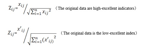
(2) Nondimensionalize the index The original data matrix with the same trend was normalized to eliminate the influence of indicator measurement units, and the normalized matrix Z was established, the naturalization process is carried out according to the following formula.(see Formula 1 in the Supplemental Files.)
The normalized matrix Z is:
Z=

Determine the positive and negative ideal solutions:
According to the normalized matrix Z, the positive ideal solution Z+ ( the optimal vector) and the negative ideal solution Z- (the worst vector) were calculated:
Positive Ideal Solution:Z+=(0.0675,0.0256,0.3063,0.1608,0.1225,0.1504,0.2633,0.2767,0.0437,0.1641,0.1991)
Negative Ideal Solution:Z-=(0.0355,0.0440, 0.1272,0.1969,0.1968,0.1990,0.0217,0.2235,0.0437,0.0556,0.1009)
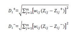
(3) Calculate the Ci value of Euclidean distance and relative proximity Calculate the Euclidean distance Di+ and Di- of the evaluation object index value and the positive and negative ideal solutions according the following formula: (see Formula 2 in the Supplementary Files)
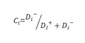
Based on the calculated Euclidean distance, the Ci value of the index value of the evaluation object, which was relatively close to the positive ideal solution and negative ideal solution, was calculated by the following formula. The Ci value is taken as the evaluation result of the medical service capacity of the key clinical specialties at the county level, which is between 0 and 1, and the specialty with the largest Ci is the best. (see Formula 3 in the Supplementary Files)
1.2.3 Rank Sum Ratio (RSR) The RSR refers to the average of the rank of a row or column. The basic idea is to obtain the statistical RSR by rank transformation in n evaluation objects and m evaluation indexes matrix. Then, parameter statistical analysis is used to study the distribution of RSR, and the RSR value is used to grade the evaluation objects directly.
1.2.4 Analysis of Influence Factors The Ci value of TOPSIS was used as the dependent variable for the analysis of influencing factors, and 13 variables were selected from the indicators in the questionnaire as the independent variables for the analysis, which is as shown in Table 3. Simple linear regression was used to screen the influencing factors of medical service capability. The variables considered as influencing factors in the simple linear regression model were incorporated into the multiple linear regression model to determine the influencing factors, and the test level was a=0.05.
Table 3 Influencing Factors
|
Level 1 Variable |
Level 2 Variable |
Code |
|
The Basic Information of The Hospital |
population in the county |
V1 |
|
Specialist basic conditions |
construction period investment total |
V2 |
|
net usable area of each bed |
V3 |
|
|
specialist actual open number of beds |
V4 |
|
|
doctor to nurse ratio |
V5 |
|
|
patient to nurse ratio |
V6 |
|
|
specialist talent team |
proportion of the average annual number of expert visits |
V7 |
|
number of technical promotion project training courses |
V8 |
|
|
number of technical promotion trainees |
V9 |
|
|
number of sent trainees |
V10 |
|
|
medical quality |
proportion of drugs |
V11 |
|
coincidence rate of main clinical diagnosis and pathological diagnosis |
V12 |
|
|
scientific research |
number of papers in core or national journals |
V13 |
2.1 TOPSIS Comprehensive Evaluation Results
The specialty A12 is of the highest comprehensive score of the first 30 county-level clinical key medical service capacity (Ci=0.94840), and specialty A14 is of the lowest (Ci=0.02147), as detailed in Table 4.
Table 4 Comprehensive Score of The capacity of The Specialty Medical Services
|
Specialist NO. |
D+ |
D- |
Ci |
Sort |
|
Specialist No. |
D+ |
D- |
Ci |
Sort |
|
A1 |
0.08891 |
0.08895 |
0.50009 |
8 |
|
A16 |
0.13519 |
0.11174 |
0.45251 |
14 |
|
A2 |
0.09273 |
0.10096 |
0.52124 |
6 |
|
A17 |
0.14151 |
0.09600 |
0.40418 |
24 |
|
A3 |
0.11401 |
0.08381 |
0.42366 |
19 |
|
A18 |
0.15708 |
0.20182 |
0.56233 |
3 |
|
A4 |
0.11161 |
0.07935 |
0.41552 |
22 |
|
A19 |
0.13296 |
0.09806 |
0.42448 |
18 |
|
A5 |
0.08018 |
0.05820 |
0.42056 |
20 |
|
A20 |
0.10117 |
0.06557 |
0.39325 |
26 |
|
A6 |
0.11743 |
0.08699 |
0.42554 |
17 |
|
A21 |
0.27744 |
0.29792 |
0.51779 |
7 |
|
A7 |
0.07634 |
0.07037 |
0.47963 |
10 |
|
A22 |
0.13009 |
0.09721 |
0.42767 |
16 |
|
A8 |
0.08906 |
0.06104 |
0.40666 |
23 |
|
A23 |
0.10507 |
0.11707 |
0.52701 |
5 |
|
A9 |
0.18414 |
0.15537 |
0.45763 |
13 |
|
A24 |
0.10051 |
0.05262 |
0.34363 |
28 |
|
A10 |
0.12430 |
0.08425 |
0.40398 |
25 |
|
A25 |
0.10970 |
0.35048 |
0.76161 |
2 |
|
A11 |
0.10467 |
0.08998 |
0.46228 |
12 |
|
A26 |
0.10945 |
0.06031 |
0.35527 |
27 |
|
A12 |
0.00529 |
0.09722 |
0.94840 |
1 |
|
A27 |
0.11635 |
0.08438 |
0.42038 |
21 |
|
A13 |
0.12718 |
0.11567 |
0.47631 |
11 |
|
A28 |
0.19059 |
0.18795 |
0.49651 |
9 |
|
A14 |
0.09721 |
0.00213 |
0.02147 |
30 |
|
A29 |
0.10039 |
0.08268 |
0.45165 |
15 |
|
A15 |
0.10842 |
0.12784 |
0.54111 |
4 |
|
A30 |
0.11912 |
0.06205 |
0.34248 |
29 |
2.2 RSR and Grouping Results
According to the Ci, the frequency f of Ci was calculated, as well as the cumulative frequency number of the f and the cumulative frequency p(R/n). As shown as Table 5. The p will be converted into the probability unit Probit (Probit=u+5, u is the standard normal deviation corresponding to p). With Probit, the probability unit value corresponding to the cumulative frequency p, as the independent variable, and Ci as the dependent variable, linear regression equation was calculated. According to Ci, the medical service capacity of 30 specialties was classified and grouped.
Table 5 Frequency distribution of Ci and the Probability Units and Sorting
|
Specialty |
Ci |
f |
Σf |
R |
p(%) |
Probit |
|
Specialty |
Ci |
f |
Σf |
R |
p(%) |
Probit |
|
A14 |
0.02147 |
1 |
1 |
1 |
3.33 |
2.77 |
|
A29 |
0.45165 |
1 |
16 |
16 |
53.33 |
5.07 |
|
A30 |
0.34248 |
1 |
2 |
2 |
6.67 |
3.16 |
|
A16 |
0.45251 |
1 |
17 |
17 |
56.67 |
5.18 |
|
A24 |
0.34363 |
1 |
3 |
3 |
10.00 |
3.5 |
|
A9 |
0.45763 |
1 |
18 |
18 |
60.00 |
5.26 |
|
A26 |
0.35527 |
1 |
4 |
4 |
13.33 |
3.89 |
|
A11 |
0.46228 |
1 |
19 |
19 |
63.33 |
5.34 |
|
A20 |
0.39325 |
1 |
5 |
5 |
16.67 |
4.03 |
|
A13 |
0.47631 |
1 |
20 |
20 |
66.67 |
5.44 |
|
A10 |
0.40398 |
1 |
6 |
6 |
20.00 |
4.16 |
|
A7 |
0.47963 |
1 |
21 |
21 |
70.00 |
5.53 |
|
A17 |
0.40418 |
1 |
7 |
7 |
23.33 |
4.26 |
|
A28 |
0.49651 |
1 |
22 |
22 |
73.33 |
5.62 |
|
A8 |
0.40666 |
1 |
8 |
8 |
26.67 |
4.38 |
|
A1 |
0.50009 |
1 |
23 |
23 |
76.67 |
5.73 |
|
A4 |
0.41552 |
1 |
9 |
9 |
30.00 |
4.47 |
|
A21 |
0.51779 |
1 |
24 |
24 |
80.00 |
5.84 |
|
A27 |
0.42038 |
1 |
10 |
10 |
33.33 |
4.56 |
|
A2 |
0.52124 |
1 |
25 |
25 |
83.33 |
5.97 |
|
A5 |
0.42056 |
1 |
11 |
11 |
36.67 |
4.66 |
|
A23 |
0.52701 |
1 |
26 |
26 |
86.67 |
6.13 |
|
A3 |
0.42366 |
1 |
12 |
12 |
40.00 |
4.74 |
|
A15 |
0.54111 |
1 |
27 |
27 |
90.00 |
6.18 |
|
A19 |
0.42448 |
1 |
13 |
13 |
43.33 |
4.82 |
|
A18 |
0.56233 |
1 |
28 |
28 |
93.33 |
6.5 |
|
A6 |
0.42554 |
1 |
14 |
14 |
46.67 |
4.92 |
|
A25 |
0.76161 |
1 |
29 |
29 |
96.67 |
6.83 |
|
A22 |
0.42767 |
1 |
15 |
15 |
50.00 |
5 |
|
A12 |
0.94840 |
1 |
30 |
30 |
99.17* |
7.39 |
*: The value was calculated according to the formula(1-1/4n)*100%
Based on the correlation and regression analysis, Ci and Probit were highly correlated, and Pearson correlation coefficient was 0.889, P<0.001. The regression equation is Ci=-0.06+0.123Probit(F=105.431,P<0.001). The batch of specialized medical service ability was classified into three groups according to the comprehensive score. The comprehensive score of medical and health service ability of the first group was the highest, followed by that of the second group and the third group. The difference among the three groups was statistically significant, as shown in the Table 6.
Table 6 Subcategory of The Capacity of Clinical Key Specialty Medical Services in Henan Province
|
Group |
Px |
Probit |
Ci |
Split Sort Result |
|
Ⅰ |
<P15.866 |
<4 |
<0.552 |
A14,A30,A24,A26 |
|
Ⅱ |
P15.866~ |
4~ |
0.0.552~ |
A20,A10,A17,A8,A4,A27,A5,A3,A19,A6, A22,A29,A16,A9,A11,A13,A7,A28,A1,A21,A2 |
|
Ⅲ |
P84.134~ |
6~ |
~0.798 |
A23,A15,A18,A25,A12 |
2.3 Analysis on The Influencing Factors of The County Level Clinical Key Specialty Medical Service Ability
2.3.1 Simple Linear Regression Analysis Among the 13 variables selected according to the indicatiors in the questionnaire of this study, 12 variables have statistically significant effects on the comprehensive score of medical service ability (P<0.05), including V1, V2, V3, V4, V5, V6, V7, V9, V10, V11, V12,V13, as shown in Table 7.
Table 7 Simple Linear Regression Analysis
|
Code |
Variable |
Regression coefficient |
P Value |
95%CI |
|
V1 |
population in the county |
0.004 |
0.000* |
(0.003,0.005) |
|
V2 |
construction period investment total |
0.000271 |
0.006* |
(0.000085,0.000457) |
|
V3 |
net usable area of each bed |
0.052 |
0.000* |
(0.043,0.060) |
|
V4 |
specialist actual open number of beds |
0.004 |
0.000* |
(0.003,0.004) |
|
V5 |
doctor to nurse ratio |
0.160 |
0.000* |
(0.126,0.194) |
|
V6 |
patient to nurse ratio |
0.214 |
0.001* |
(0.101,0.327) |
|
V7 |
proportion of the average annual number of expert visits |
0.006 |
0.000* |
(0.005,0.007) |
|
V8 |
number of technical promotion project training courses |
0.005 |
0.083 |
(-0.001,0.011) |
|
V9 |
number of technical promotion trainees |
0.000 |
0.000* |
(0.000158,0.000419) |
|
V10 |
number of sent trainees |
0.025 |
0.000* |
(0.014,0.037) |
|
V11 |
proportion of drugs |
0.013 |
0.000* |
(0.010,0.015) |
|
V12 |
coincidence rate of main clinical diagnosis and pathological diagnosis |
0.005 |
0.000* |
(0.004,0.005) |
|
V13 |
number of papers in core or national journals |
0.026 |
0.000* |
(0.016,0.037) |
PS: * stands for P<0.05, and the difference is statistically significant.
2.3.2 Multiple Linear Regression Analysis The 12 variables considered as influencing factors in the results of simple linear regression analysis were incorporated into the multiple linear regression model and analyzed by the entry method. The results showed that, V2, V3, V6, V9, V12, a total of 5 variables had a statistically significant impact on the medical service capacity of key clinical specialties at the county level (P<0.05), and details seen in Table 8.
Table 8 Multiple Linear Regression Analysis
|
Code |
Variable |
Regression Coefficient |
P Value |
95%CI |
|
V1 |
population in the county |
0.001 |
0.489 |
(-0.001,0.002) |
|
V2 |
construction period investment total |
-0.000154 |
0.014* |
(-0.00027,-0.000038) |
|
V3 |
net usable area of each bed |
0.017 |
0.002* |
(0.008,0.026) |
|
V4 |
specialist actual open number of beds |
-0.002 |
0.057 |
(-0.005,0.001) |
|
V5 |
doctor to nurse ratio |
0.070 |
0.072 |
(-0.008,0.149) |
|
V6 |
patient to nurse ratio |
-0.315 |
0.023* |
(-0.578,-0.052) |
|
V7 |
proportion of the average annual number of expert visits |
0.000011 |
0.988 |
(-0.002,0.002) |
|
V9 |
number of technical promotion trainees |
0.000 |
0.006* |
(0.000049,0.000228) |
|
V10 |
number of sent trainees |
0.008 |
0.162 |
(-0.004,0.021) |
|
V11 |
proportion of drugs |
0.001 |
0.768 |
(-0.004,0.005) |
|
V12 |
coincidence rate of main clinical diagnosis and pathological diagnosis |
0.005 |
0.001* |
(0.002,0.007) |
|
V13 |
number of papers in core or national journals |
0.003 |
0.384 |
(-0.005,0.012) |
PS: F=70.962,P<0.001;R2=0.989,Adjusted R2=0.972,MSE=0.006,Model is meaningful and well-fitting; * stands for P<0.05, and the difference is statistically significant.
The 13th five-year health and health development plan of Henan Province emphasizes that priority should be given to the development of county-level hospitals, with the goal of basically preventing serious diseases from leaving the county, according to the principle of supplementation and consolidation, strengthening the construction of common diseases, frequently-occurring diseases and key specialties as well as related specialties, and comprehensively improving the capacity of medical services in the county [6]. In this study, the medical service ability and corresponding influence factors of the county level clinical key specialty were evaluated in Henan province, and it has been discovered that, there is an imbalance in the development of the capacity of the 30 key specialties in terms of medical services when the construction cycle is completed, and the basic conditions (total amount of funds invested during the construction period, net use area of beds, ratio of bed care), the effect of medical quality (clinical primary diagnosis, pathological diagnosis compliance rate), talent training (number of technical promotion trainees) have a significant effect on medical service capacity. Therefore, it is necessary to further strengthen the management of the construction projects of the county-level clinical key specialties, and the specialist heads should also make reasonable plans for the development.
3.1 Ensure the basic configuration meets the needs of residents’ health care services
During the 11th five-year plan period, Henan province vigorously promoted the construction of county-level medical and health service system and implemented the plan of doubling the service capacity of county-level hospitals, so that the total amount of health resources of county-level hospitals continued to increase and the allocation of beds and other infrastructure facilities gradually improved. The allocation and utilization of bed resources in a region is an important index to measure the development of health services [7]. The net use area of the batch of the specialty in Henan Province averaged 6.005 ㎡ [8], and the average bed utilization rate was 88.00% [9], which can be considered to be in line with the needs of health services in the region, and not wasted, according to the implementation plan of the construction of clinical key specialty projects, the net use area of beds should be greater than or equal to 6 ㎡. The average patient to nurse ratio for the batch of the specialty is 1:0.7 [8], and the indicator has achieved the target of “the second-level hospital patient to nurse ratio will reach 1:0.5 by 2020”, proposed in outline of China’s nursing career development plan (2016-2020). Therefore, the allocation of health resources in nursing staff, beds and the like can meet the needs of residents in the county area, commendably.
3.2 Guarantee the investment of specialized funds to create conditions for personnel training and medical technology upgrading
During the “11th Five-Year Plan” period, the construction of basic configuration of count-level hospitals in Henan Province provided a solid hardware foundation for the development of their medical service capacity. During the “12th Five-Year Plan” period, the construction project of key clinical specialties at the county level in Henan Province was launched to promote the transformation of project units from the extensive development of scale expansion to the construction of specialized personnel training teams and strengthening of connotation construction [10]. The county-level hospital and the specialty should pay more attention to the development of appropriate medical technology level of health talents and the input of soft power such as medical quality; use project funds reasonably and efficiently, and improve the health service capacity of county-level medical institutions comprehensively.
3.2.1 Strengthen talent training and enhance comprehensive capabilities The limited development speed of the specialized medical service ability of county-level hospitals is related to the unreasonable talent team structure. Although the talent introduction has been strengthened, most county-level hospitals adopt the mode of reemployment after retirement and expert support from superior hospitals, and still lack high-level talents and academic leaders. At the same time, aging knowledge of some health workers, due to financial problems, lacking of learning and opportunities, slow the development of their service capacity. During the construction of the clinical key specialty in Henan province, a group of talents with master’s degree or above have been introduced, which have strong ability and innovation ability. The department should make reasonable use of the project funds, strengthen the connection with the superior hospital, tap the talent potential of the specialized department, provide excellent talents with opportunities and channels for further study in the superior hospital, help them update their knowledge and skills, and expand their scope of knowledge; in addition, in order to meet the demand of diagnosis and treatment of common diseases frequently-occurring disease, which is taken as a starting point, specialized subject should cooperate with the superior hospitals, carry out clinical technology research, improve specialized talents clinical ability and innovation ability, cultivate a group of specialized subject, form a team, to further improve the comprehensive ability of specialized subject.
3.2.2 Increase the promotion of appropriate technology With the deepening of the reform and construction of medical consortium, various forms of cooperation have been formed among provincial , city level hospitals and county hospitals, which not only closes the contact between the hospital at the county level and superior medical units ,but can make it be able to quickly solve various medical problem, more facilitate the promotion and application of appropriate technologies in county hospitals, and is an important approach to enhance the level of county hospital medical technology. With the increasing awareness of health care among the people, the diversified and multi-level needs of residents put forward new requirements for medical and health services. Due to the lack of scientific and reasonable plan for the use of funds, the promotion and application of appropriate technology are limited to a certain extent in county hospitals. More paths should be explored for the specialties , with the support of provincial (municipal) hospitals, training courses on appropriate technology promotion should be held to boost the promotion and application of appropriate health technology for common diseases and health problems, so as to help health workers strengthen their understanding and grasp of new technology and improve their clinical skills, build special brand, upgrade the level of specialty technology and gradually alleviate the imbalance of development among urban and rural regions, which could reduce the waste of health resources caused by insufficient technical capacity, to some extent, and lighten the economic burden of local residents due to disease, and promote the balanced development of medical service system simultaneously,.
3.3 Ensure the quality of health care all along
Medical quality is an important part of the development of health services in China, which affects the people’s use of health rights and utilization of medical services. The results of this study show that the coincidence rate of clinical diagnosis and pathological diagnosis influences medical service ability statistically, which is consistent with relevant research. The average clinical diagnostic coincidence rate of the batch of the specialty was 98.25%, and which is not less than 95% in the implementation plan of the county-level clinical key specialties in Henan province. The batch of specialty represented the high level of provincial county-level hospitals at the initial stage of construction with high medical quality, and could still show its benchmark level in the province after construction of 3 years. The specialty should perfect the medical service supervision system and strengthen the monitoring and supervision upon the quality and safety of medical service behavior; and improve the medical quality control system and facilitate the safety as well as the effectiveness of medical services to a higher degree. Meanwhile, quantitative evaluation on the department’s business activities should be carried out, the execution of the system should be ensured. It is crucial to heighten the department staff’s sense of responsibility to ensure the quality, and promote the medical quality to achieve the goal of sustainable development.
Since 2012, China has promoted the comprehensive reform of county-level public hospitals. At present, Zhejiang Province, Henan Province, Shanxi Province, Sichuan Province and Hubei Province have established the project of provincial-county clinical key specialty. There have been scholars who have put forward opinions and suggestions on the construction of county-level clinical key clinical specialties, but there is a lack of evaluation and analysis on the construction based on empirical data and quantitative indicators. On the basis of relevant data collection, this study makes a comprehensive evaluation of the capacity of the first batch of county-level clinical key specialty medical services in Henan Province by establishing the index system and TOPSIS method, and provides quantitative results for further analysis of factors. Through linear regression analysis, the factors influencing medical service capacity were screened and determined, so as to scientifically and effectively analyze the deficiencies and problems existing in the construction of the specialty, and put forward targeted suggestions. The combination of TOPSIS method and linear regression method can be effectively applied to the study of comprehensive capacity evaluation and influence factor analysis of medical institutions.
5.1 Ethics approval and consent to participate
Not applicable. This study does not involve biological and pharmaceutical experiments, and there are no ethical issues.
5.2 Consent for publication
Not applicable.
5.3 Availability of data and materials
The data that support the findings of this study are available on request from the corresponding author [Henan Medical Association]. The data are not publicly available due to [state restrictions e.g. “them containing information that could compromise research participant privacy/consent”]. The raw data involved in this study shows that in the article.
5.4 Competing interests
The authors declare that they have no competing interests.
5.5 Abbreviation
TOPSIS Technique for Order Preference by Similarity to an Ideal Solution
5.6 Funding
This research program belongs to Henan Medical Science And Technology Project, and it was funded by Henan Medical Association. Henan Medical Association was committed by Health Commission of Henan Province to conduct questionnaire survey and project evaluation. The data and information in the manuscript were obtained and supported through the questionnaire survey conducted by Henan Medical Association.
5.7 Author’s contributions
Wang Z.L, Sun N, Bi C.X and Ma X.S were responsible for the distribution and recovery of questionnaires. Li M.J sorted the data. Wang W and Zhao S.C managed project implementation and progress. Guo J.L designed the subject and analyzed the data. Wang K.X analyzed the data and was the a major contributor in writing the manuscript. All authors read and approved the final manuscript.
5.8 Acknowledgements
Appreciate the support of Henan Medical Association for its assistance in the process of questionnaire distribution and data collection.
- Shi Lei, Xiao Jian-Xia, Hu Kai, Ma Nan, Yin Shan-Shan, Zong Shang-Wei, Nie Wei. Analysis of the status quo of the declared project of the construction of the key clinical specialty at the county level in Henan Province. Henan Medical Research, 2015(10):59-61.http://www.wanfangdata.com.cn/details/detail.do?_type=perio&id=hnyxyj201510027
- Gou Zheng-Xian. Study on The Evaluation Index System of Clinical Key Specialty in Chengdu County-Level Hospitals. Chongqing Medical University, 2014. https://kns.cnki.net/KCMS/detail/detail.aspx?dbcode=CMFD&dbname=CMFD201501&filename=1014409571.nh&v=MDIwOTRIZ1VidklWRjI2R3JlNEY5VExycEViUElSOGVYMUx1eFlTN0RoMVQzcVRyV00xRnJDVVJMT2VaZWR2Rnk=
- Niu Xiao-Hui. Construction and Research of Evaluation Index System of National Key Clinical Specialties in Shanxi Province, Shanxi Medical University, 2017. https://kns.cnki.net/KCMS/detail/detail.aspx?dbcode=CMFD&dbname=CMFD201801&filename=1017848529.nh&v=MDU0MTFPcHBFYlBJUjhlWDFMdXhZUzdEaDFUM3FUcldNMUZyQ1VSTE9lWmVkdkZ5SGdWci9CVkYyNkdidThGdFQ=
- Wan Guang-Sheng, Qian Zhi-Wang, Shi Yu-Feng, et al. Evaluation of Medical and Health Services in The Pearl River Delta Cities Based on Ahp-TOPSIS Method. Chinese Health Economics, 2017,36(12):95-97. http://www.wanfangdata.com.cn/details/detail.do?_type=perio&id=zgwsjj201712028
- Zhang Xiao-Lin, Jiao Ming-Li, Wang Guo-Dong, et al. Analysis of Government-Related Responsibilities in The New Health Care Reform in A Province Based on TOPSIS Law. Chinese Health Economics, 2015,34(06):22-24. http://www.wanfangdata.com.cn/details/detail.do?_type=perio&id=zgwsjj201506007
- Henan Political Office. A Notice on The Issuance of The Health And Health Development Plan of Henan Province’s 13th Five Year Plan. 2017. https://www.henan.gov.cn/2017/01-25/248702.html
- Gong Han-Xiang, Wu Ze-Yong, Wu Bao-Ling, et al. Evaluation And Analysis of Spatial Aggregation Characteristics of Medical And Health Resources in Guangdong Province. Chinese Health Economics, 2017,36(05):52-55. http://www.wanfangdata.com.cn/details/detail.do?_type=perio&id=zgwsjj201705016
- Wang Kai-Xuan, Guo Jin-Ling, Wang Wei, et al. Analysis of Key Clinical Specialists at County-Level in Henan Province. Chinese Journal of Hospital Administration, 2018, 34(11):918-921. http://www.wanfangdata.com.cn/details/detail.do?_type=perio&id=zhyygl201811009
- Wang Kai-Xuan, Wang Wei, Zhao Shui-Chang, et al. Analysis on The Development of Key Clinical Specialty Medical Service Capacity at County Level in Henan Province.. Chinese Hospital Management, 2019,39(02):37-40. http://www.wanfangdata.com.cn/details/detail.do?_type=perio&id=zgyygl201902014
- Zhang Feng. Henan Makes The County Clinical Key Specialized Subject stronger. 2017. http://health.china.com.cn/2019-01/03/content_40632356.htm
- Huang Ju, Yu Chen, Zhang Lu. Influence of Soft Budget Constraint on Service Delivery Behavior of Public Hospitals: An Empirical Analysis Based on County-Level Public Hospitals. Chinese Health Economics, 2016, 35(05):22-24. https://kns.cnki.net/KCMS/detail/detail.aspx?dbcode=CJFQ&dbname=CJFDLAST2016&filename=WEIJ201605007&v=MDMxNjBGckNVUkxPZVplZHZGeUhoVUwzTE1pakNaTEc0SDlmTXFvOUZZNFI4ZVgxTHV4WVM3RGgxVDNxVHJXTTE=
- Tian Di, Zhou Yuan, Zhou Dian. Evaluation of A Hospital’s Medical Quality (2012-2016) Based on Rank And Ratio And Multiple Association Methods. Chinese Journal of Health Statistics, 2018, 35(01):80-82. https://kns.cnki.net/KCMS/detail/detail.aspx?dbcode=CJFQ&dbname=CJFDLAST2018&filename=ZGWT201801022&v=MDAwMDhIOW5Ncm85SFpvUjhlWDFMdXhZUzdEaDFUM3FUcldNMUZyQ1VSTE9lWmVkdkZ5SGhVTHZPUHlyY2VyRzQ=
- Zhang Li-Ping, Yu Zhen-Jie, Li Wang-Chen, et al. The Design And Empirical Study of The Comprehensive Evaluation Scheme of Medical Quality Based on The Comparison of Different Methods. Chinese Journal of Health Statistics, 2016,33(01)_:158-160. https://kns.cnki.net/KCMS/detail/detail.aspx?dbcode=CJFQ&dbname=CJFDLAST2016&filename=ZGWT201601053&v=MjU1NDFyQ1VSTE9lWmVkdkZ5SGhVYnpKUHlyY2VyRzRIOWZNcm85QVo0UjhlWDFMdXhZUzdEaDFUM3FUcldNMUY=
- Tao Yuan, Gao Yang-Fang, Zhou Yue, et al. Comprehensive Evaluation of The Quality of Medical Treatment in Clinical Departments by TOPSIS and RSR Based on The Main Component Analysis Method. Chinese Journal of Health Statistics, 2016, 33(02):324-326. https://kns.cnki.net/KCMS/detail/detail.aspx?dbcode=CJFQ&dbname=CJFDLAST2016&filename=ZGWT201602047&v=MTMzNjdlWmVkdkZ5SGhVYnZBUHlyY2VyRzRIOWZNclk5Qlk0UjhlWDFMdXhZUzdEaDFUM3FUcldNMUZyQ1VSTE8=
- Zhang Zhi-Qiang, Xiong Ji-Xia. Systematic Dynamics Analysis of The Factors Influencing The Comprehensive Performance of Public Hospitals. Chinese Health Economics, 2015, 34(03):76-79. https://kns.cnki.net/KCMS/detail/detail.aspx?dbcode=CJFQ&dbname=CJFDLAST2015&filename=WEIJ201503026&v=MDIxNzk4ZVgxTHV4WVM3RGgxVDNxVHJXTTFGckNVUkxPZVplZHZGeUhoVjdySU1pakNaTEc0SDlUTXJJOUhZb1I=