The availability of only scalar data obviously complicates the procedure for reconstructing the total magnetic field vector. The concomitant Backus effect mentioned above can be eliminated by adding the knowledge of the accurate location of the magnetic dip equator [Khokhlov et al., 1997]. Its minimization is basically gained in one of three ways:
-
adding relevant vector data especially collected in the equatorial belt (e.g., [Cain et al., 1967]);
-
adding observations of the position of the equatorial electrojet [Holme et al., 2005];
-
taking into account the position of the dip equator derived from the reference model [Ultré-Guérard et al., 1998].
For reducing the Backus effect, we follow the third way as the IGRF model is available for epochs 1964 and 1970. Using this model, we determine the dip equator position at each degree of the longitude for the middle of the satellite operation period. To construct a magnetic field model, we adopt formula (4) from [Ultré-Guérard et al., 1998] and minimize the function
$$S(g,h)=\sum _{i=1}^{M}{w\left({\mathbf{r}}_{i}\right)\left({B}_{i}-B({\mathbf{r}}_{{i}};g,h)\right)}^{2}+{w}_{eq}\sum _{j=1}^{N}{Z({\mathbf{r}}_{j};g,h)}^{2}.$$
Here M is the number of measurements, \({B}_{i}\) are the values of the measured total field, \({\mathbf{r}}_{i}\) are the points at which the measurements were made, \(B({\mathbf{r}}_{i};g,h)\) is the total field value according to the model with a set of Gauss coefficients \({g}_{nm},{h}_{nm}\), \(w\left({\mathbf{r}}_{i}\right)\) is a weighting factor aimed to balance the different density distribution of the measurements over the Earth's surface, N is the number of points \({\mathbf{r}}_{j}\) defining the dip equator, \(Z({\mathbf{r}}_{j};g,h)\) is the Z component value according to the model at those points and \({w}_{eq}\) is the weight applied to the dip equator constraint. For a LEO satellite with a maximum trajectory latitude \({\theta }_{\text{m}\text{a}\text{x}}\), the weighting factor \(w\left({\mathbf{r}}_{{i}}\right)\) chosen as \(\sqrt{{\text{sin}}^{2}{\theta }_{\text{m}\text{a}\text{x}}-{\text{sin}}^{2}\theta }\) takes into account the fact that most of the measurements are concentrated near the latitudes \({\pm \theta }_{\text{m}\text{a}\text{x}}\). For the sparse measurements, the weighting factor can be omitted. As for \({w}_{eq}\), the result of minimization is practically independent of this factor within a wide range (two orders of magnitude). In our calculations, we take \({w}_{eq}\) equal to 100.
The actual minimization is carried out by the built-in function lsqnonlin () of the Matlab package, which enables solving nonlinear least-squares (nonlinear data-fitting) problems. The minimization method is iterative. The subsequent step of minimizing the function \(S\left(x\right)=\frac{1}{2}{\sum }_{i}^{ }{f}_{i}^{2}\left(x\right)\) is performed in the two-dimensional subspace of the parameter space spanned by the gradient of the function \({g}_{k}={\sum }_{i}^{ }{f}_{i}^{ }\frac{\partial {f}_{i}}{\partial {x}_{k}}\) at a given point and the Newtonian step n, which is determined from the system of equations
$$\sum _{p}^{ }\sum _{i}^{ }\frac{\partial {f}_{i}}{\partial {x}_{k}}\frac{\partial {f}_{i}}{\partial {x}_{p}}{n}_{p}=-{g}_{k}.$$
A function in a two-dimensional subspace is approximated by a quadratic form. If the next calculated step leads to a decrease in the function value, then follows the next iteration. If not, the admissible step decreases, and the procedure is repeated. Calculation stops when the admissible step becomes small enough. As an initial approximation, the values of the coefficients \({g}_{nm},{h}_{nm}\) are chosen according to the IGRF model at the beginning of 1965 and 1970.
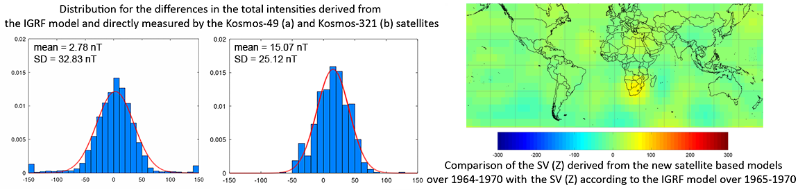
To calculate the coefficients based on the Kosmos-49 (hereinafter referred to as the “N-1” model) and Kosmos-321 (hereinafter, the “N-2” model) data, we apply weakened selection criteria than those used for comparing measurements with the IGRF model (see Section 2). This is due to the extremely small set of raw measurements, especially those obtained by the Kosmos-321 satellite; if they are filtered according to the criteria specified in Section 2, we get vast regions of Africa, Europe and Canada that are not covered by data at all (see Fig. 1b).
Thus, when selecting data from the Kosmos-49 satellite, the time filter is removed and only the criteria Kp ≤ 2 and |Dst| < 20 nT are applied. We also discard the evident erroneous measurements visible on the histogram in Fig. 2a as bars on the left and right for residuals of more than 150 nT. As a result, 12511 out of 17499 measurements are used for building the N-1 model. Mean and SD of the differences between the N-1 model and the actual observations are 0.23 nT and 27.57 nT, respectively (see Table 1). Maps with plotted positions of the Kosmos-49 satellite when taking the measurements selected for the N-1 model are shown in Fig. 7a.
For data selection from the Kosmos-321 satellite, we apply the latitudinal filter |lat| < 60o and weakened criteria Kp ≤ 3 and |Dst| < 50 nT. As a result, 2311 out of 4910 measurements remain; their spatial distribution is shown in Fig. 7b. Mean and SD of the differences between the N-2 model and the actual observations are 0.56 nT and 15.70 nT, respectively (see Table 1). The coefficients of the resulting two models are listed in Tables 4–5.
Table 4
Gauss coefficients of the new geomagnetic field model based on the measurements from the Kosmos-49 satellite (“N-1”); the coefficients are listed in three columns.
| \({n}\) | \({m}\) | \({{g}}_{{n}{m}}\) | \({{h}}_{{n}{m}}\) | \({n}\) | \({m}\) | \({{g}}_{{n}{m}}\) | \({{h}}_{{n}{m}}\) | \({n}\) | \({m}\) | \({{g}}_{{n}{m}}\) | \({{h}}_{{n}{m}}\) |
| 1 | 0 | -30410 | 0 | 5 | 4 | -162 | -99 | 8 | 1 | 12 | 3 |
| 1 | 1 | -2120 | 5775 | 5 | 5 | -63 | 80 | 8 | 2 | -6 | -14 |
| 2 | 0 | -1656 | 0 | 6 | 0 | 51 | 0 | 8 | 3 | -8 | 5 |
| 2 | 1 | 3001 | -2020 | 6 | 1 | 70 | -21 | 8 | 4 | -3 | -20 |
| 2 | 2 | 1595 | 113 | 6 | 2 | 6 | 102 | 8 | 5 | 6 | 5 |
| 3 | 0 | 1184 | 0 | 6 | 3 | -226 | 68 | 8 | 6 | -3 | 23 |
| 3 | 1 | -2046 | -403 | 6 | 4 | 2 | -35 | 8 | 7 | 11 | -3 |
| 3 | 2 | 1297 | 234 | 6 | 5 | 0 | -10 | 8 | 8 | 4 | -18 |
| 3 | 3 | 853 | -164 | 6 | 6 | -114 | -8 | 9 | 0 | -6 | 0 |
| 4 | 0 | 961 | 0 | 7 | 0 | 26 | 0 | 9 | 1 | 8 | -27 |
| 4 | 1 | 817 | 140 | 7 | 1 | -56 | -68 | 9 | 2 | 6 | 10 |
| 4 | 2 | 481 | -271 | 7 | 2 | 8 | -33 | 9 | 3 | -16 | 7 |
| 4 | 3 | -391 | 16 | 7 | 3 | 9 | -4 | 9 | 4 | 11 | 0 |
| 4 | 4 | 253 | -270 | 7 | 4 | -25 | 9 | 9 | 5 | 2 | -4 |
| 5 | 0 | -297 | 0 | 7 | 5 | -3 | 24 | 9 | 6 | -1 | 9 |
| 5 | 1 | 353 | 9 | 7 | 6 | 15 | -23 | 9 | 7 | 3 | 10 |
| 5 | 2 | 254 | 123 | 7 | 7 | -1 | -13 | 9 | 8 | 1 | 0 |
| 5 | 3 | -32 | -126 | 8 | 0 | 14 | 0 | 9 | 9 | -1 | 1 |
Table 5
Gauss coefficients of the new geomagnetic field model based on the measurements from the Kosmos-321 satellite (“N-2”); the coefficients are listed in three columns.
| \({n}\) | \({m}\) | \({{g}}_{{n}{m}}\) | \({{h}}_{{n}{m}}\) | \({n}\) | \({m}\) | \({{g}}_{{n}{m}}\) | \({{h}}_{{n}{m}}\) | \({n}\) | \({m}\) | \({{g}}_{{n}{m}}\) | \({{h}}_{{n}{m}}\) |
| 1 | 0 | -30219 | 0 | 5 | 4 | -162 | -87 | 8 | 1 | 7 | 8 |
| 1 | 1 | -2078 | 5733 | 5 | 5 | -53 | 79 | 8 | 2 | -3 | -18 |
| 2 | 0 | -1779 | 0 | 6 | 0 | 46 | 0 | 8 | 3 | -12 | 5 |
| 2 | 1 | 3001 | -2037 | 6 | 1 | 60 | --16 | 8 | 4 | -6 | -14 |
| 2 | 2 | 1604 | 19 | 6 | 2 | 19 | 105 | 8 | 5 | 7 | 4 |
| 3 | 0 | 1258 | 0 | 6 | 3 | -212 | 70 | 8 | 6 | 2 | 20 |
| 3 | 1 | -2101 | -363 | 6 | 4 | 3 | -42 | 8 | 7 | 8 | -9 |
| 3 | 2 | 1282 | 251 | 6 | 5 | 1 | -2 | 8 | 8 | 5 | -14 |
| 3 | 3 | 839 | -203 | 6 | 6 | -108 | -1 | 9 | 0 | -1 | 0 |
| 4 | 0 | 961 | 0 | 7 | 0 | 57 | 0 | 9 | 1 | 11 | -21 |
| 4 | 1 | 802 | 170 | 7 | 1 | -60 | -72 | 9 | 2 | 4 | 15 |
| 4 | 2 | 459 | -269 | 7 | 2 | 3 | -28 | 9 | 3 | -14 | 4 |
| 4 | 3 | -393 | 30 | 7 | 3 | 16 | -4 | 9 | 4 | 10 | -4 |
| 4 | 4 | 235 | -286 | 7 | 4 | -24 | 9 | 9 | 5 | -1 | -2 |
| 5 | 0 | -231 | 0 | 7 | 5 | 1 | 19 | 9 | 6 | -2 | 11 |
| 5 | 1 | 365 | 27 | 7 | 6 | 13 | -22 | 9 | 7 | 7 | 12 |
| 5 | 2 | 261 | 138 | 7 | 7 | 0 | -12 | 9 | 8 | 0 | -1 |
| 5 | 3 | -38 | -144 | 8 | 0 | 18 | 0 | 9 | 9 | -1 | 2 |
The comparison of the N-1 and N-2 models with the IGRF model (Z component) for the epochs 1964 and 1970 is shown in Fig. 8. An expected degradation in the data approximation by the N-2 model is observed in those parts of the African continent (Fig. 8b) where original data are missing (see Fig. 7b). Nevertheless, as compared to M-1 and M-2 models, N-1/N-2 deviations from the IGRF predictions are reduced significantly.
An improvement in the SV prediction for the indicated epochs can be traced by comparing the discrepancy between the M-1/M-2 and IGRF models (Fig. 6) with the discrepancy between the N-1/N-2 and IGRF models. Figure 9 shows a map for the latter case, limited to ± 60о in latitude due to the same limitation for the initial data selection for the N-1/N-2 models. The SV according to the new models becomes more realistic in the eastern part of the Pacific Ocean, African continent and the vast region of Southeast Asia (see Figs. 6 and 9). In general, Fig. 9 demonstrates modest variance in SV predictions between N-1/N-2 and IGRF models. We estimate the SV predicted by different modes more in detail in the next section.