We asked if genes that first appeared in a particular phylostratum were always distributed at random across the chromosomes of living animals, or were there perhaps contributions from particular phylostrata in which we see such genes distributed preferentially to a specific chromosome. In Figure 1, the leftmost figure shows the % of “great ape” genes (phylostratum 19.2); the middle figure shows the “fish” genes (phylostratum 12), in both cases as they are distributed across the autosomal human chromosomes, while the rightmost figure shows the phylostratum 12 genes of the zebrafish (Danio rero) which, being a jawed fish, appears itself in phylostratum 12. The data that we report are, across the chromosomes of the specified animal species, the number of genes recruited in a particular phylostratum as a percentage of the total number of genes present on each chromosome, normalized by being divided by the median across that phylostratum:
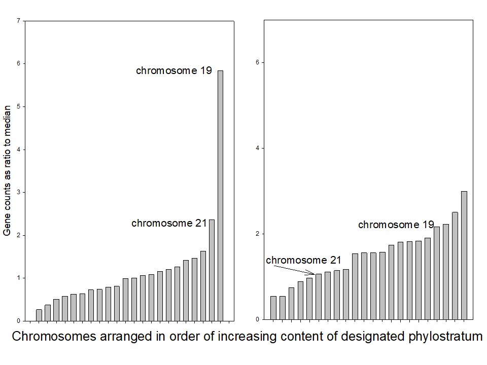
It can be seen, comparing the leftmost and middle figures, that the genes that were acquired with the appearance of the great apes (with a MAD +/- SEM value of 0.38+/- 0.09, n=22) are far more unevenly distributed among the human chromosomes than are the genes that were acquired with the emergence of the fish (0.05+/- 0.01, n=22). The difference is significant at P<0.05 (Holm-Sidak Pairwise Multiple Comparison). Comparing the middle and right figures of 1 shows that the phylostratum 12 genes are, similarly, evenly distributed also among the chromosomes of the fish itself where the MAD +/- SEM has a value of 0.08+/- 0.02, n=25), the difference between these two distributions being non-significant using the same statistical test. The spread between the 75% and 25% limits as a function of the median in each case is 0.13 for the “fish” genes in the human genome while being 0.73 for the “great ape” genes. The two chromosomes with the highest fraction of phylostratum 19.2 genes (left figure, these being chromosomes 21 and 19) are no longer the most enriched compared with the phylostratum 12 genes (middle figure, where chromosome 21 is now 7th from the top and chromosome 19, 13th).
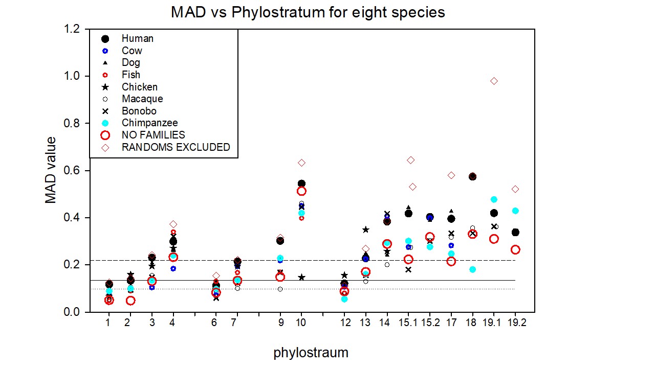
Extending this same approach, we studied the random/non-random distribution of newly appearing genes, phylostratum by phylostratum, across the full evolutionary trajectory for eight animal species chosen from a range of phylostrata. Figure 2 shows the results of this analysis, plotted as the Mean Absolute Deviation about the Median (MAD – see Methods), divided by the medians, against phylostratum number for these eight animal genomes, each animal species being shown by a different symbol. (The red circles in the figure denote the data for the human genome from which we removed all the genes that belong to a number of gene families. These results will be considered later in the paper). The raw data and computations upon which this figure is built are presented as Tables S2 through S10 in the Supplementary Materials). Note the structure of this plot: There are three data points (other than the red circle) for phylostratum 19.2, depicting the genes added in phylostratum 19.2 for the three great apes that we have analysed. Phylostratum 19.1 shows four data points, the genes that were added in phylostratum 19.1 for the three great ape species plus the data point for the macaque monkey (Macaca mulatta) that represents for us phylostratum 19.1. As successively earlier phylostrata are considered, further data points are added at each earlier phylostratum until, from phylostratum 12 and earlier, all eight points appear at each phylostratum number, one from each of the eight species that we have used. We performed the analysis using only the autosomal genes since we were concerned that the intense evolution of, especially, the Y chromosome in the more recent phyla might affect the results. (The analysis using the whole chromosome complement is very similar to Figure 2 (data not shown)). The horizontal lines drawn are the median, and the 25% and 75% limits, computed for all the data through to phylostratum 12, the euteleostomii (the jawed fish).
Using a mixed-effects model (from the Non Linear Mixed Effect package of R), accounting for the repeated measure element of retesting species, the MAD values for the tetrapoda (phylostratum 13) do not differ significantly (at P= 0.3711) from those for the combined phylostrata 1 through 12, but significance holds (at P< 0.0001) for all of the more recent phylostrata. The values for the olfactores at phylostratum 10 lie significantly above the data for the combined phylostrata 1 through 12, P< 0.0001). This is in spite of the extensive chromosomal rearrangements that have taken place since the time that the olfactores appeared (See the Discussion for more in such chromosomal arrangements). The contribution of the olfactores to the human genome is only 85 genes out of more than 19,000. With such a small sample number, their distribution among the 22 to 25 (in different species) autosomal chromosomes might be expected to be somewhat uneven, and variable from species to species. Indeed, the correlation coefficient between the human and macaque data for phylostratum 10 genes is not significant at P=0.57, whereas that for the 19.1 phylostratum between these two species is less than 0.0001. If these outlying olfactores data are excluded from the combined phylostrata 1 through 12, the MAD values for the tetrapoda are now significantly different from those of the combined phylostrata 1 through 12 at P=0.024.
It would appear from these data that during the evolution of the vertebrates, from the amniota (and possibly the tetrapoda) through to the great apes, the distribution of newly recruited genes across the chromosomes appears as being increasingly non-random. An important message from this plot is this: If one looks at the MAD value for the genes that emerged with, for example, the amniotes (at phylostratum 14), their MAD number does not differ much when those “amniote” genes are seen in the chromosomes of the chicken itself, or those of the chimpanzee, macaque, or dog chromosomes. A distribution of that particular degree of scatter is found in the chromosomes of the amniotes through to the great apes, although the chromosomes themselves have evolved and today vary so much between the species in size and number.
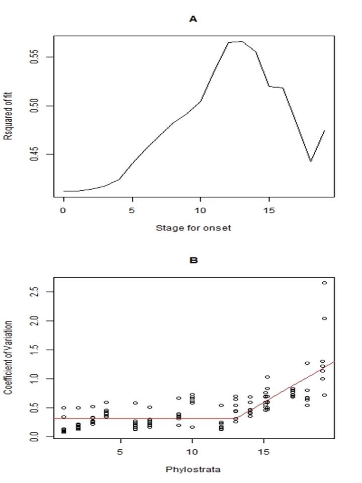
We tested whether the data could perhaps best be described by two straight lines, one horizontal and the other with a delayed slope, an ascending function of phylostratum age. An appendix in the Supplementary Methods provides the results of such an analysis. The delayed slope model was significantly superior to a single slope (p<0.001).
We wondered whether the increasing patchiness seen for the newly recruited genes might in part arise from a preferred localisation to those chromosomes that had preferentially recruited genes during the immediately previous phylostratum. Table 2 records as a matrix the Spearman rank order correlations between the distributions of newly recruited genes across all the chromosomes, phylostratum by phylostratum. Phylostratum names, as rows and columns, are in bold. The correlation between the chromosome distribution of the genes of any phylostratum X and the distribution of those of the succeeding phylostrata, is given as the point of intersection between the rows and columns of the matrix, and is displayed as the correlation coefficient r and, directly below this, the corresponding probability P. All correlations that have P<0.05 are in bold type.
|
TABLE 2 Spearman correlation coefficients of (autosomal) chromosome distributions between successive phylostrata in Homo sapiens (Bold-type values have coefficients with P< 0.05)
|
|
|
|
|
|
13
|
14
|
15.1
|
15.2
|
17
|
18
|
19.1
|
19.2
|
|
12
|
0.0446
|
0.161
|
-0.27
|
-0.211
|
-0.29
|
-0.143
|
-0.395
|
-0.549
|
|
P value
|
0.84
|
0.469
|
0.22
|
0.342
|
0.188
|
0.521
|
0.0681
|
0.00823
|
|
|
|
|
|
|
|
|
|
|
|
13
|
|
-0.0198
|
-0.0593
|
-0.0491
|
0.162
|
0.0209
|
0.283
|
0.18
|
|
P value
|
|
0.928
|
0.789
|
0.825
|
0.466
|
0.924
|
0.199
|
0.417
|
|
|
|
|
|
|
|
|
|
|
|
14
|
|
|
0.135
|
0.0288
|
-0.00395
|
-0.215
|
0.239
|
-0.246
|
|
P value
|
|
|
0.544
|
0.896
|
0.984
|
0.332
|
0.28
|
0.266
|
|
|
|
|
|
|
|
|
|
|
|
15.1
|
|
|
|
0.65
|
0.248
|
0.0503
|
0.383
|
0.434
|
|
P value
|
|
|
|
0.00104
|
0.262
|
0.821
|
0.077
|
0.0431
|
|
|
|
|
|
|
|
|
|
|
|
15.2
|
|
|
|
|
0.659
|
0.309
|
0.278
|
0.24
|
|
P value
|
|
|
|
|
0.000817
|
0.159
|
0.206
|
0.278
|
|
|
|
|
|
|
|
|
|
|
|
17
|
|
|
|
|
|
0.606
|
0.23
|
0.233
|
|
P value
|
|
|
|
|
|
0.00286
|
0.299
|
0.292
|
|
|
|
|
|
|
|
|
|
|
|
18
|
|
|
|
|
|
|
0.303
|
0.435
|
|
P value
|
|
|
|
|
|
|
0.167
|
0.0425
|
|
|
|
|
|
|
|
|
|
|
|
19.1
|
|
|
|
|
|
|
|
0.557
|
|
P value
|
|
|
|
|
|
|
|
0.00719
|
It will be noticed that most of the highest correlations are between successive phylostrata. These are significant except between phylostrata 18 and 19.1, where the correlation is below significance, although the correlation between phylostrata 18 and 19.2 is significant (as is that between 19.1 and 19.2). Table S11, in the Supplementary Materials shows the similar results, again for Homo sapiens, but now using the restricted set of more consistent data for which 3 or more ortholog databases agreed with the modal value
We extended these between-phylostrata correlations to include a number of mammalian species. The full data set can be found as Table S12 of the Supplementary Materials.
We had noted in Figure 1 that phylostratum 19.2 has the highest percentage of newly recruited genes on chromosome 19. We asked whether the location of newly recruited genes along chromosome 19 itself might correlate with the location of the genes recruited in the previous phylostratum. To test this, we divided chromosome 19 into twenty successive equal sections of gene counts (This gave 70 genes in each section except for the 69 genes that remained for the twentieth section). In each section, we computed the proportion of genes from any phylostratum X in chromosome 19 as a percentage of the genes of phylostratum X in the whole genome. We then performed Spearman rank order phylostratum to phylostratum correlations between the gene distributions along the twenty successive sections across chromosome 19. We asked whether the section by section content of phylostratum X genes along the chromosome correlated with the distribution of the succeeding phylostrata. The part of the data that show significant correlations is depicted in Table 3. The table records as a matrix the Spearman rank order correlations between the distribution of newly recruited genes across the twenty sections of chromosome 19, phylostratum by phylostratum. Phylostratum names appear as the rows and columns of the table. The correlation between any two phylostrata is given as the point of intersection between the rows and columns of the matrix, and is displayed as the correlation coefficient r and, below this, the corresponding probability P. All correlations that have P<0.05 are in bold type, the single correlation with P=0.051 is in italics.
Table 3
Spearman correlation coefficients of distributions along the twenty sections of chromosome 19, between successive phylostrata _ Homo sapiens (Bold type values have coefficients with P< 0.05, italicized value P=0.051)
|
|
|
15.2
|
17
|
18
|
19.1
|
19.2
|
|
. 151
|
0.31
|
-0.132
|
-0.167
|
-0.232
|
0.0561
|
|
P value
|
0.18
|
0.572
|
0.476
|
0.32
|
0.811
|
|
15.2
|
|
0.14
|
-0.0253
|
-0.35
|
-0.184
|
|
P value
|
|
0.551
|
0.911
|
0.127
|
0.429
|
|
17
|
|
|
0.458
|
0.3
|
0.0921
|
|
P value
|
|
|
0.0414
|
0.194
|
0.695
|
|
18
|
|
|
|
0.44
|
0.199
|
|
P value
|
|
|
|
0.051
|
0.396
|
|
19.1
|
|
|
|
|
0.698
|
|
P value
|
|
|
|
|
0.00051
|
|
|
|
|
|
|
|
Thus, significant (at P<0.05) correlations exist between the distributions along the twenty sections of chromosome 19 of phylostrata 17 and 18, and 19.1 with 19.2 and a borderline significant correlation (P=0.51) between 18 and 19.1. The correlations between non-successive phylostrata are not significant.
We wanted to find out if there was a particular region of chromosome 19 at which these new gene additions, phylostratum to previous phylostratum, occurred. We used a heat map showing the gene content of the successive 20 sections of chromosome 19, comparing successive phylostrata, to provide the answer. The heat map (built as a percentage of the genes of a particular phylostratum, in a particular section, to all the genes of that phylostratum in the entire genome) is depicted in the upper part of Figure 3:
The Zinc Finger (ZNF) genes of chromosome 19.
It would appear that the distal half of the q portion of chromosome 19 (the most distal four sections in particular) are the richest in genes that originated in recent phylostrata (17 through 19.2), those that showed the highest between- phylostrata correlations in chromosomal distributions (Table 3). Section 20 (at the distal section of the q arm of the chromosome) appears on Figure 3 as a section with a high content of both phylostrata 17 and 19.1. This section contains a high proportion of zinc finger (ZNF) genes, these being 65% of all the genes in this section of chromosome 19. Chromosome 19 contains a high proportion of ZNF genes. Indeed, of its 1396 protein-coding genes 248 or almost 18% are ZNF genes. Figure 4A below depicts the ZNF genes of the human genome as a function of phylostratum number and chromosome location.
As can be seen, the ZNF genes are in general, recent, with most of them having been recruited in phylostrata 17 and 19 (the hoofed and pawed animals and the primates, respectively). It is apparent, too, that chromosome 19 is to a very large extent the preferred location for these genes. We have seen that it is the most distal section of the q arm of this chromosome that is especially preferred. The distribution across chromosome 19 of the ZNF genes as a percentage of all the ZNF genes of the genome was depicted as a heat map in the lower half of figure 4. The map to map comparison is striking. The location of the successive cohorts of newly recruited ZNF genes appears, in many cases, to be coordinated. All of the phylostratum 19.2 genes are located at the sites where 19.1 genes had been formed, and many of the phylostratum 19.1 genes locate close to phylostratum 17 genes.
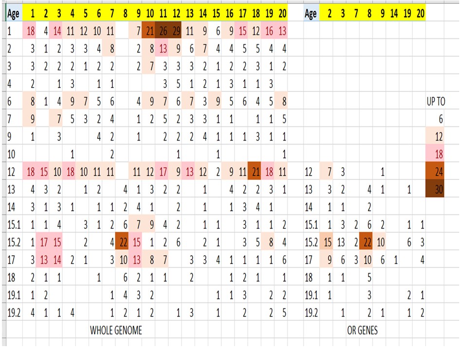
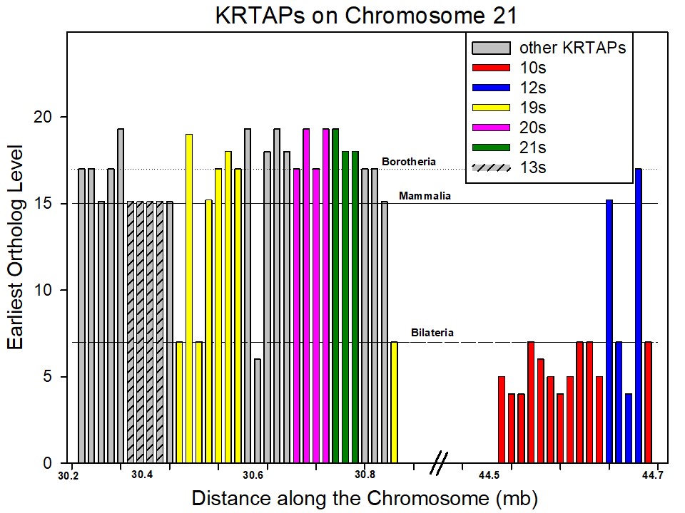
Keratin-associated protein (KRTAP) genes. We looked for a second gene family that could be involved in between-phylostrata relations. In Figure 1, the chromosome with the highest proportion of phylostratum 19.2 genes is chromosome 21. Now chromosome 21 is rich in genes from the KRTAP (Keratin Associated Protein) family. Figure 4B depicts the distribution of the KRTAP family genes by phylostratum age and by chromosomal location. Over 50% of these genes are located on chromosome 21 and a very high proportion of them are recent genes, largely arising with the mammals. The KRTAP genes are associated with the evolution and development of hair, a mammalian innovation(7). The KRTAP gene family can be divided into numerous sub-families of shared evolutionary history(8), and Supplementary Figure S2 depicts these sub-families as they are situated on chromosome 21
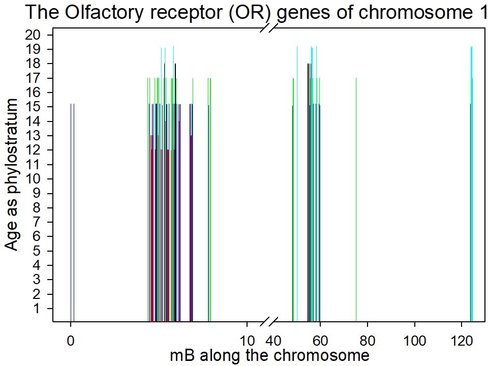
The Olfactory Receptor (OR) genes. As an additional gene family we chose the OR genes, the olfactory receptor genes. There are 406 of these in the human genome. Figure 4C shows their distribution by age and by chromosome location. Chromosome 11 is by far the richest bearer of the OR genes. Most of the OR genes were recruited with the first mammals, next highest being the hoofed and pawed animals of phylostratum 17. Supplementary Figure S3 shows the location of the OR genes along human chromosome 11. The OR genes are indeed non-randomly distributed, being present in two major complexes, with a few other solitary cases. The major complex, in the proximal region between 4.5 and 6 mB, is centered around the genes that were recruited in phylostratum 12, with the genes from phylostrata 15, 17, 18 and 19 being close by. Many of the more recent genes of chromosome 11, these being for the most part mammalian genes, were contributed by the Olfactory receptor (OR) gene family. Our prior familiarity with the ZNF, KRTAP, and OR gene families led to their being chosen as convenient samples of the class.
Increase in randomness with evolutionary time after excluding the gene families.
In addition to the three major gene families, the ZNF, KRTAP, and OR families, there are a number of minor gene families that we surmised might contribute to the non-randomness of gene distributions among the chromosomes. These minor families include the TRAV family of 45 genes, all located on chromosome 14, the TRBV family of 37 members on chromosome 7, the KIR2D and KIR3D families with 45 genes on chromosome 19, the LILR family with 33 genes on chromosome 19, and the NLRP family of 15 genes, 9 of which are located on chromosome 19. These latter genes are associated with the adaptive immune response which began to evolve with the origin of the jawed fish(9). In addition, we took account of the PCDH gene family of 66 members, 55 of which are on chromosome 5. This list consists of the genes in those families that contain ten or more members and comprises 923 genes.
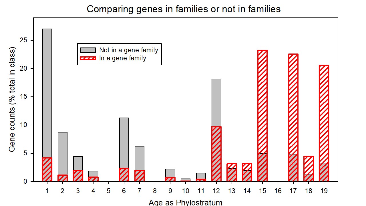
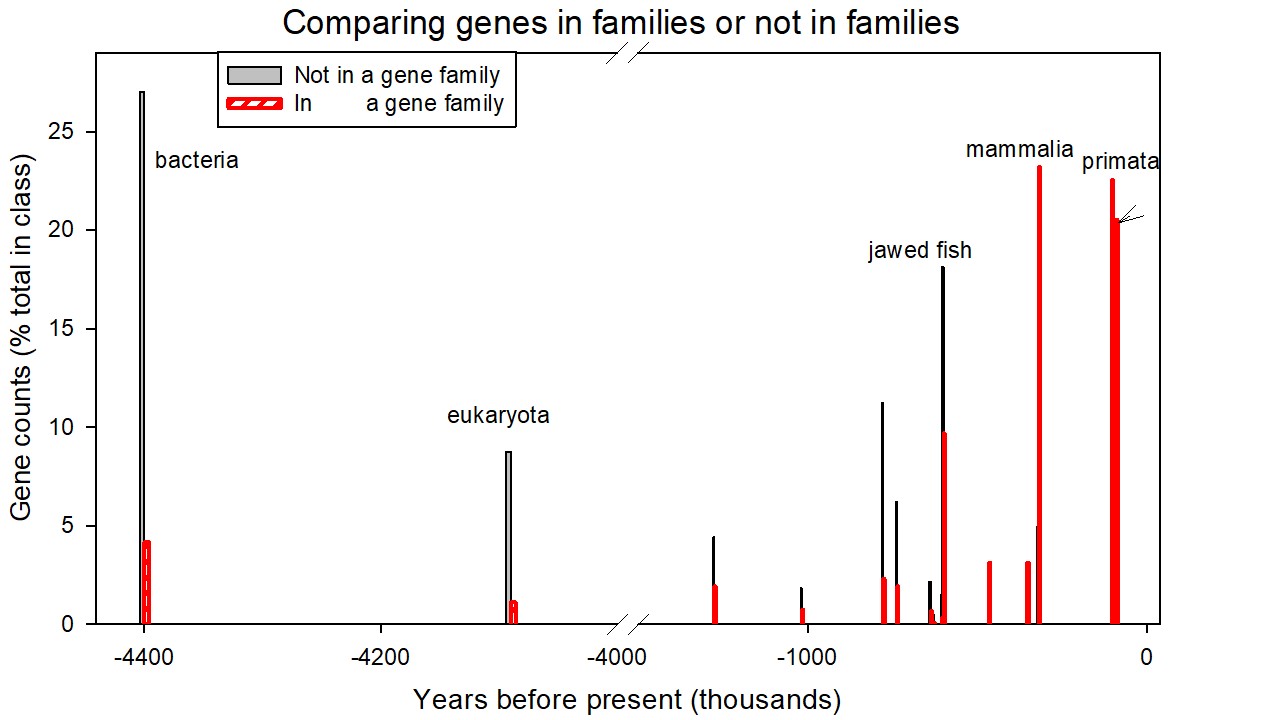
The genes that were incorporated into the evolving human genome as members of a gene family did so at much later epochs than those that were incorporated as an individual. Table S13 in the Supplementary Materials lists these two classes of genes together with their consensus ages while Figures S4 and S5 in the Supplementary Materials depict these data plotted as the percentage of genes of that class (the set incorporated into families or the set incorporated as individuals) as a function of consensus age (depicted as phylostratum number in S4 or as thousands of years before present in S5). The two distributions, analysed by the Mann-Whitney Rank Sum Test (with medians of 6 and 15.2 in consensus ages) were statistically different at p<0.001. It would appear that, from the tetrapoda onwards, comparing the two sets, the fraction of newly-added genes that were incorporated into gene families did so significantly later than the fraction of those incorporated as individuals. At each phylostratum, the fraction of genes incorporated into a family as a proportion of all genes so incorporated increases linearly with phylostratum number (p= 0.010) while, in contrast, the fraction incorporated as individuals shows an insignificant decrease.
We wondered whether excluding all the genes that were incorporated into families might diminish the bunching of newly added genes that we had seen in Figure 2 and thus asked what the MAD versus phylostratum plot might look like after excluding these major and minor gene families. The red circles in Figure 2S in the Supplementary materials depict a plot of the uneven distribution of genes across the chromosomes of the human genome, calculated again as the appropriate MAD values, but now after excluding 923 genes, this being the total of the genes contributed by all the above-cited families. The open red triangles depict a control in which we excluded a random sample of 923 of the genes of the human genome and calculated again the appropriate MAD values.
The data points computed for the human genome after excluding these gene families differ little from the other data points until the tetrapoda are reached, but then the data for the full genomes deviate increasingly upwards. This parallels the increasing fraction of genes that are in gene families which begins to deviate upwards at much the same time period (Figure S4). The difference between the MAD values for the full human genome, for genes that were added from the tetrapoda and later, is significantly different (P=0.001, t-test, N=7) from the data where the gene families are excluded. The difference between the MAD values for the full human genome is not significantly different (P=0.301, t-test, N=17) from the data where 923 genes were excluded at random. By extending the Non Linear Mixed Effect regression model to include the set with 923 randomly-excluded genes, this set could be shown to be significantly different (P=0.0017, from the data set in which the gene families were excluded.
The MAD values where the gene families are excluded remain, from the amniota onwards, significantly different (at P = 0.02, Mann-Whitney Rank Sum Test) from the data set of the MAD values through the jawed fish at phylostratum 12. This residual variance, which does not seem to arise from bunching by the previously-listed gene families, will be considered further in the discussion.
We wondered whether or not it would be useful to consider, during a particular phylostratum, the genes that were added to families already in the evolving genome separately from those genes that were added as non-related individuals. To that end we chose all the 874 genes added as the primate clade evolved and divided these into the 417 genes that appear in the gene families listed previously (Supplementary Table S14, worksheet 2) and the remaining 457 that were added as individuals (Supplementary Table S14, worksheet 3). Figure S6A in the Supplementary Materials shows that those genes that were recruited to the evolving primate genome as members of an existing gene family) are very unevenly distributed among the chromosomes with a MAD value of 0.52, whereas primate genes that were added as individuals were evenly distributed, with a MAD value of 0.26 (Figure S6B).