We utilized the vertical component of continuously recorded seismic waveforms by permanent and temporary stations from April 1 to September 30 during the year 2019. The permanent stations included 78 Hi-net stations, 1 Kyushu University station, 1 Tokyo University station, 2 Nagoya University stations, 10 AIST stations, 16 Kyoto University stations and 9 JMA stations, and temporary stations comprised 104 Kyoto University Manten project stations (Iio et al. 2018; Katoh et al. 2019), that are distributed around the central part of the Kinki region. Combining these set of stations enabled us to obtain a dataset with adequate short-period surface waves ray paths coverage and a subsequent 3D S-wave velocity model of high-resolution. Firstly, we computed the cross-correlation of ambient noise to extract surface waves propagating between pairs of seismic stations. We then estimated Rayleigh wave phase velocity measurements between station pairs using the zero-crossing method (Ekström et al. 2009). Finally, we constructed the shallow crustal 3D S-wave velocity structure by applying the direct surface wave inversion method (Fang et al. 2015).
Surface wave phase velocity measurements
Phase velocity measurements can be conducted in either the time domain or frequency domain. The time domain analysis requires the high-frequency approximation and only considers those interstation distances exceeding three wavelengths (λ) (Bensen et al. 2007; Lin et al. 2008; Yao et al. 2006). In contrast, the frequency domain approach has no theoretical limitation for interstation distances (i.e., zero-crossing method; Ekström et al. 2009). As such, interstation distances up to approximately one wavelength can be practically used (Ekström et al. 2009; Tsai and Moschetti 2010). In our study, we used the zero-crossing method to derive phase velocity measurements between station pairs. This method is based on modeling cross-correlation spectra by the spatial autocorrelation (SPAC) method (Aki 1957; Asten 2006) and uses the zero-crossing frequencies of the real part of the cross-correlation spectra. The SPAC method is premised on the assumption that ambient noise sources are homogeneously distributed and that ambient noise is predominantly surface waves (Aki 1957). Under this assumption, a Bessel function of the first kind and zeroth order can be used to model the real part of the vertical cross-correlation spectra as follows:
\(Real\left(\rho \left(f,x\right)\right)= {J}_{0}\) (\(\frac{2\pi fx}{{C}_{R}\left(f\right)}),\) (1)
where \(\rho\) is the cross-spectrum, f is the frequency, x represents the interstation distance, J0 represents the Bessel function of the first kind and zeroth order, and CR(f) represents the Rayleigh wave phase velocity. In the zero-crossing method, we only focus on the zero crossing points where both sides of Eq. (1) should be zero. The zero-crossing points are not sensitive to fluctuations in the power spectrum of the background noise and non-linear filtering in the data processing (Ekström et al. 2009). Using zero crossings simplifies phase velocity measurements and stabilizes the estimation of phase velocities because phase velocity estimation is not affected by incoherent noise (Cho et al. 2021).
If fn represents the frequency of the observed nth zero crossing point of the cross-correlation spectrum, and Zn denotes the nth zero of the Bessel function, we can match each fn with the zero crossing points of the Bessel function to have all the possible phase velocity dispersion curves according to the following equation:
$${C}_{m}\left({f}_{n}\right)= \frac{2\pi {f}_{n}x}{{Z}_{n+2m}},$$
2
where m representing the number of missed or additional zero crossing points, takes the values (0, ±1, ±2,…). Applying Eq. (2) for all observed values of fn yields numerous possible dispersion curves.
We used the GSpecDisp package (Sadeghisorkhani et al. 2018) to estimate phase-velocity dispersion curves uniquely by the zero-crossing method from the stacked cross-correlations. To reduce noise effects in the correlations, we applied a velocity filter of 1–4.5 km/s with a taper interval of ~0.2 km/s. Then, we applied spectral whitening to each correlation for amplitude equalization (Sadeghisorkhani et al. 2018). With many possible phase velocities occurring at each frequency with regard to Eq. (2) (colored dots; Fig. 3a), it is difficult to uniquely determine the phase velocity dispersion curves without using a reference velocity dispersion curve as a guide. To circumvent this, we manually picked the dispersion curve appearing closest to the reference dispersion curve. In the GSpecDisp, average velocities can be estimated by combining all cross-correlation spectra (average velocity module). We estimated average velocities in the period range from 2 to 8 s and used the result as a reference velocity for dispersion curve estimation in single station-pair phase-velocity picking mode in GSpecDisp (dashed black dots; Fig. 3a). Finally, we estimated phase-velocity dispersion curves between all the possible station pairs (red circles in Fig. 3a).
For our dataset, the maximum measurable period required an interstation distance (x, in km) of at least three wavelengths (λ), defined as the r/λ ratio in GSpecDisp (x/λ ≥ 3). For each cross-correlation function, the signal-to-noise ratio (SNR) was defined as the ratio between maximum absolute amplitude in the signal window (between arrival times corresponding to waves with 1 and 4.5 km/s) and the root mean square amplitude in the noise time window (between 500 and 700 s). We used an SNR threshold of 10 to reject correlations with low signal. Finally, we obtained a total of 23,647 dispersion curves (Fig. 3c).
Direct inversion of the surface wave dispersion curves
Ambient noise tomography using phase velocity dispersion curves typically involves a two-step procedure. Firstly, 2D phase velocity maps are constructed by travel-time tomography at discrete frequencies. Secondly, pointwise inversion of dispersion data for 1D profiles of S-wave velocity as a function of depth at each grid point is implemented, and combining multiple 1D profiles subsequently yields the 3D S-wave velocity structure (Shapiro and Ritzwoller 2002; Yao et al. 2008). Nonetheless, a 3D S-wave velocity structure can equally be estimated by direct inversion of dispersion data without the intermediate step of constructing 2D phase velocity maps (Boschi and Ekström 2002; Fang et al. 2015; Feng and An 2010; Pilz et al. 2012). Typically, these direct inversion approaches do not update the ray paths and sensitivity kernels for the newly constructed 3D models (Fang et al. 2015). Also, one-step linearization may produce biased wave velocity estimations in a medium akin to the shallow crustal structure, where S-wave velocity variations can exceed 20% (Lin et al. 2013).
To estimate the 3D S-wave velocity structure from phase velocity dispersion data, we applied a direct surface wave tomography method (DSurfTomo), which is based on frequency-dependent ray-tracing and a wavelet-based sparsity-constrained inversion (Fang et al. 2015). This approach circumvents the intermediate step of constructing 2D phase velocity maps and iteratively updates the sensitivity kernels of period-dependent dispersion data (Fang et al. 2015). Furthermore, it accounts for the ray-bending effects of period-dependent ray paths by using the fast-marching method (Rawlinson and Sambridge 2004). Accounting for such effects in the inversion is especially useful for short-period surface waves, which are significantly sensitive to the highly complex shallow crustal structure (Fang et al. 2015; Gu et al. 2019). Therefore, this approach is a well-suited tool for determining the shallow-crustal structure of the Kinki region using short-period surface-waves dispersion data.
In tomographic inversion, the objective is to find a model m that minimizes the differences \(\delta {t}_{i}\left(f\right)\) between the measured travel times \({t}_{i}^{obs}\left(f\right)\) and the calculated travel times \({t}_{i}\left(f\right)\) from the model for all frequencies \(f\). The travel time for path \(i\) is given as
$${\delta t}_{i}\left(f\right)= {t}_{i}^{obs}\left(f\right)- {t}_{i}\left(f\right)\approx -\sum _{k=1}^{K}{v}_{ik}\frac{{\delta C}_{k}\left(f\right)}{{C}_{k}^{2}\left(f\right)},$$
3
where \({t}_{i}\left(f\right)\) represents the computed travel times from a reference model which can be updated during the inversion, \({v}_{ik}\) denotes the bilinear interpolation coefficients along the ray path associated with the ith travel-time data, \({C}_{k}\left(f\right)\) is the phase velocity and its perturbation \({\delta C}_{k}\left(f\right)\) at the k-th two-dimensional surface grid node at frequency \(f\) (Fang et al. 2015). Surface wave dispersion is primarily sensitive to S-wave velocity. However, short-period Rayleigh wave dispersion is also sensitive to the compressional (P-wave) velocity in the shallow crustal structure (Fang et al. 2015). The P-wave velocity perturbations together with mass density are therefore explicitly included in the calculation of surface wave dispersion, with \({R}_{\alpha }^{\text{'}}\) and \({R}_{\rho }^{\text{'}}\) as scaling factors, leading to the following equation:
$${\delta t}_{i}\left(f\right)= \sum _{k=1}^{K}\left(-\frac{{v}_{ik}}{{C}_{k}^{2}}\right)\sum _{j=1}^{J}{\left.\left[{R}_{\alpha }^{\text{'}}\left({z}_{j}\right)\frac{{\partial C}_{k}}{{\partial \alpha }_{k}\left({z}_{j}\right)}+ {R}_{\rho }^{\text{'}}\left({z}_{j}\right)\frac{{\partial C}_{k}}{{\partial \rho }_{k}\left({z}_{j}\right)}+ \frac{{\partial C}_{k}}{{\partial \beta }_{k}\left({z}_{j}\right)}\right]\right|}_{{\theta }_{k}}{\delta \beta }_{k}\left({z}_{j}\right) = \sum _{l=1}^{M}{G}_{il}{m}_{l}$$
4
,
where \({\theta }_{k}\) denotes the one-dimensional (1D) reference model at the k-th surface grid node, \({\alpha }_{k}\left({z}_{j}\right)\), \({\rho }_{k}\left({z}_{j}\right)\), and \({\beta }_{k}\left({z}_{j}\right)\) represent the P-wave velocity, the mass density, and the S-wave velocity, respectively. J indicates the number of grid points in the depth direction, and \(M=KJ\) represents a sum of all the model grid points. Equation (4) can be written as follows:
d = Gm, (5)
where d, G, and m represent the surface wave travel-time residual vector for all ray paths and discrete frequencies, data sensitivity matrix, and the model parameter vector, respectively. We applied the damping and weighting parameters are applied to balance data fitting and smoothing regularization. In addition to the damping and weighting parameters, the sparsity fraction, which is a parameter indicating how sparse the sensitivity matrix is, was selected on a trial-and-error basis for our data considering the diverse patterns in inverted S-wave velocity models (weakly smoothed and strongly smoothed S-wave velocity models are shown in Figures S1 and S2, respectively).
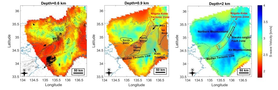
In our inversion, the entire Kinki region was parameterized into 55 by 60 grid points on the horizontal plane with 0.05° intervals between grid points in each horizontal direction, as well as 7 grid points along the depth direction (i.e., 0, 0.5, 1.0, 2.2, 4.0, 6.0 and 9.0 km). These parameters along with the large volume of dispersion data were memory intensive, we therefore used dispersion data within a narrow frequency bandwidth of 0.083 - 0.67 Hz to circumvent the computer memory limitations during the inversion. Dispersion measurements within a broad frequency bandwidth of 0.05 - 0.95 Hz was used for the northern part of the Kinki area, which was parameterized into 29 by 96 grid points on the horizontal plane with 0.02° grid point intervals in the latitude and longitude directions, and 11 grid points along the veritical direction (0, 0.1, 0.3, 0.5, 0.8, 1.4, 2.0, 3.0, 4.0, 5.5 and 7.0 km). Empirically, the fundamental mode Rayleigh wave phase velocity is primarily sensitive to 1.1 × S-wave velocity at a depth of about 1/3 multiplied by its corresponding wavelength (λ) (Fang et al. 2015; Foti et al. 2014; Hayashi 2008). Consequently, we averaged the observed Rayleigh wave phase velocities at depths of about 1/3λ and then multiplied them by 1.1 to construct and initial S-wave velocity model of the study area (i.e., a one-third wavelength transformation; Fig. 4). To account for the influence of topography on our S-wave velocity models, we subtracted altitude value from the depth value at each grid point. Therefore, the depth shown in our final 3D S-wave velocity models is the depth below sea level (S-wave velocity models before topographic correction are shown in Figures S3, S4 and S5).