Leaf starch was determined in two independent sets (i.e., a training set and a test set) of plants grown in two separate experiments. Wet laboratory measurements were taken on exactly the same material as used for the hyperspectral measurements.
Plant material and growth conditions
Thirty red clover plants obtained from IPK Gatersleben, Seeland, Germany and Agroscope, Zurich, Switzerland, were used for the study (Additional file 1: Table S1). All plants were clonally propagated, using cuts that contained only one shoot and one root meristem to ensure comparable physiological states of all plants. These clonally propagated plants were grown in a climate chamber for 90 days before harvesting (3:2:1 soil: peat: perlite substrate, photoperiod of 14:10-h L:D, day temperature 20 ± 2 °C, night temperature 15 ± 2 °C and relative humidity, 60 ± 10%). Samples were taken at the end of the night (EN; before lights were turned on), and at the end of the day (ED; before lights were turned off). The training set included 18 randomly selected genotypes, six thereof clonally duplicated, resulting in a total of 24 plants (Additional file 1: Table S1). Starch was measured on twelve plants at EN and on twelve plants at ED, using 15 leaf cuts per plant, taken on all three leaflets of five leaves (the youngest, fully emerged leaf [y], the oldest leaf [o] and three intermediate leaves [m; Fig. 1]). In total, the training set included 360 measurements (24 plants x 3 leaflets x 5 leaves per plant). The test set included six plants from three different genotypes. Three plants were harvested at ED and three plants at EN (Additional file 1: Table S1). For the test set, ten leaf cuts were taken per plant on randomly selected leaflets of mature leaves, resulting in a total of 60 measurements (6 plants x 10 leaflets per plant).
Leaf spectroscopy
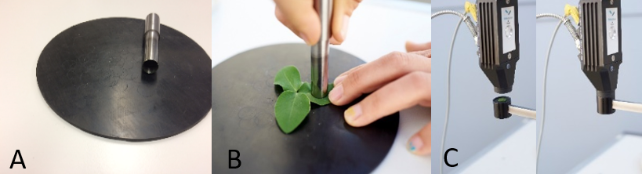
Leaflets were cut using a round, sharpened tube with a diameter of 12 mm to standardize leaf area (Additional file 2: Fig. S1). These leaf cuts were placed on the matt black surface of the FieldSpec4 pro device (Analytical Spectral Devices, Boulder, Colorado, USA). The device is not influenced by external light sources, potentially enabling the application in field experiments. Radiance between 350 and 2500 nm was measured. The spectrometer’s contact probe was fixed on a clamp, and the sample was placed so that no light escaped through the sides. Leaf samples were referenced to a spectralon white reference every fifth recording and the radiance measurements where transformed to reflectance. Immediately after taking spectral measurements, leaf cuts were flash frozen in liquid nitrogen and freeze-dried for 48 h.
After taking spectral measurements, whole plants from the training set were cut 2 cm above ground, flash-frozen and freeze-dried for starch quantification.
Wet lab analysis for starch quantification
Starch in leaf cuts and whole plants was quantified as described by Ruckle et al. [8]. Two additional clones of one genotype, not included in the correlation model, were iodine stained to visualize the starch pattern within a plant. Plants were harvested either at ED or at EN, washed with tap water and placed in 80% (v / v) boiling ethanol. After two hours, when plants were transparent, they were removed and placed in Lugol’s solution. After 10 minutes, the Lugol’s solution was rinsed off to destain the non-target areas. The plants were photographed on a light-table.
Statistical analyses
Statistical analyses were performed using the R statistical software version 3.6.0 [28]. Significance testing was performed using the library MASS [29]. Assumptions of homoscedasticity of variances and normality of residuals were not met, therefore an exact Wilcoxon rank sum test at α = 5% was performed.
Pre-processing of spectral data
Spectral analysis was realized using the R package simplerspec [30]. The mean reflectance values of 10 measurements per sample were used. Leaf spectra were pre-processed prior to modelling. Gaps between the different detector arrays at λ = 1000 nm and at λ = 1800 nm were splice corrected. Spectra were smoothed with the Savitzky-Golay first derivative filter using a 3rd-order polynomial at a 21-point window (21 nm at a resampled spectrum interval of 1nm; R package prospectr [31]). Spectral pre-processing is crucial to reduce significant noise and baseline drift resulting from light scatter before establishing a correlation model. After smoothing the spectra with Savitzky-Golay the spectral variables were centered and scaled prior to relating them to leaf starch using partial least squares regression (PLSR), in order to consider variables equally independent of their variation in absolute values. PLS regression is a substantial chemometric method, which can cope with multicollinearity in spectra and delivers robust calibration models with many predictors and few observations [32, 33]. To further reduce collinearity in processed spectra, only every forth wavelength was kept for modelling, resulting in 533 spectral predictor variables.
Model development
Leaf reflectance data from the training set was modelled by PLSR [32], using either raw or pre-processed spectra as predictors. A 5-times repeated 10-fold cross-validation scheme was used to fit the models, to determine the best number of components (ncomp), and to estimate model performance of the final model. A constant random seed was set for resampling, yielding identical hold out data across all models. Model reliability was assessed by the coefficient of determination (R2) and slope (b) of a linear regression with intercept, the root mean square error (RMSE, Eq. 1), the bias or mean error (Eq. 2), and the ratio of performance to deviation (RPD, Eq. 3). The evaluation metrics were calculated by aggregating all holdout predictions from the repeated 10-fold cross-validation (ŷi) and corresponding observed values (yi) grouped by ncomp. (see Equations 1-3 in the Supplemental Files)
Variable influence on projection scores (VIP) is a measure of variable importance tailored to PLS regression [34–36]. VIP scores were calculated from the PLS regression parameters taking multicollinearity into account, which is likely to occur because of the nature of spectroscopic data. VIP scores are considered as a robust measure to identify relevant predictors, here important wavelengths. A variable with VIP above 1 contributes more than the average variable to the model prediction. The VIP value vj was calculated for each wavelength variable j as (see Equation 4 in the Supplemental Files)
where waj are the PLS regression weights for the ath component for each of the wavelength variables and SSa is the sum of squares explained by the ath component (Eq.4). The sum of squares SSa for the ath component was calculated from the score qa of the predicted variable y and the ta scores of the spectral matrix X (Eq. 5): (see Equation 5 in the Supplemental Files)
VIP scores were also used to filter important predictors with a threshold of VIP > 1 within the training set, and the identified predictors were used to re-calibrate the test set and assess performance. This separation in the VIP filtering by independent tests was needed to avoid overfitting and over-optimistic assessment that typically occurs when identifying subsets of features on the modelling data.
In addition to the VIP based filtering, two other procedures were applied for wavelength selection. First, the 50 most relevant wavelengths to estimate starch according to Pearson’s correlation coefficient (r) were taken to re-perform PLS regression. Second, four wavelengths that were assigned to starch in previous literature were taken and normalized with the reflection at the wavelength that had the smallest standard deviation across the entire wavelength range, prior to performing a multiple linear regression (MLR; [22]).
Model evaluation using the test set
The best training model tuned by cross-validation and refitted on all training data, and the training models with three different wavelength selection (filtering) methods were tested on the independent test data set (60 samples). The predictive ability of these final models was again evaluated using R2 and RMSE on the test set. Besides these test set predictions, a PLSR model was re-calibrated using only the test data. This re-calibration allowed to determine whether the test set possibly contained different or differently weighted spectral features relevant for starch prediction, so that PLSR training relationships did not generalize to this independent test experiment.