Plant Material and Growth Conditions
One-year-old apple rootstocks of ‘Malling 7’ (‘M7’), a moderately fire blight-susceptible rootstock, were purchased from Willamette Nurseries Inc. (Canby, OR), and used in two different experiments. ‘M.7,’ a commercially important apple rootstock, was originally selected from traditional French rootstocks, known as ‘Doucin’, at East Malling Research Station (UK).
To evaluate influence of root mass of rootstocks on fire blight susceptibility of grafted scions, 45 different scion genotypes were grafted onto 1-year-old ‘M.7’ rootstocks (Supplementary Table S1). These grafted trees were maintained in a moist dark chamber for a period of three months to promote healing of the graft unions. Then, these grafted trees were planted in D40H deepots (Stuewe and Sons, Tangent, OR), 6.5 cm in diameter and 24.2 cm in depth, containing a standard Cornell soil mix (50 peatmoss:50 vermiculite with 6.2 kg.m-3 lime, 1.25 kg.m-3 superphosphate, and 0.62 kg.m3 calcium nitrate). These trees were allowed to acclimatize and grow in a greenhouse facility at Cornell AgriTech (Geneva, NY) maintained at 25°C, 50% RH, and 16 h light/8 h dark photoperiod for a period of 8 weeks. For each scion genotype, three replications were maintained in the greenhouse facility at the Cornell AgriTech (Geneva, NY), and arranged in a completely randomized block design.
To assess the effects of varying root mass (g) on fire blight susceptibility, 21 non-grafted ‘M.7’ rootstocks were used in a second experiment. One-year-1-year-old ‘M.7’ rootstocks were pruned from the bottom up, using Fiskars hedge shears, to alter the numbers of adventitious root nodes growing along each of the rootstocks. The resulting rootstocks were photo-imaged, and analyzed using ImageJ (https://imagej.nih.gov/ij/) to identify four classes (RACs) that exhibit significantly different root area from one another. These non-grafted ‘M.7’ rootstocks were then potted in plastic pots (26 cm in diameter and 22.5 cm in depth) using the Cornell Soil mix as described above. For each RAC rootstock treatment, three replications were used, and these trees were maintained in the greenhouse facility at Cornell AgriTech, arranged in a completely randomized block design, under conditions of 25°C, 50% RH, and 16 h light/8 h dark photoperiod for a period of 106 days.
Fire Blight Inoculation and Trait Evaluation
Bacterial inoculum was prepared using a highly virulent E. amylovora strain, Ea2002A. Frozen inoculum stock was transferred to a petri plate containing King’s B medium (KB), and incubated for 48 h at 28°C. Bacterial cells were recovered in a suspension culture using 1X PBS, and adjusted to a concentration of 109 CFU/ml on a SmartSpec Plus Spectrophotometer (Bio-Rad Laboratories, Hercules, CA, USA).
Potted young trees were inoculated with either bacteria (treatment) or water (control; only in second experiment) for fire blight evaluation. The youngest unfolded leaf of an actively growing shoot of a potted young tree was inoculated by bisecting across the midribs using scissors dipped in the bacterial suspension, as described earlier [38, 57]. Deionized water was used to bisect midribs of leaves of control plants in the second experiment.
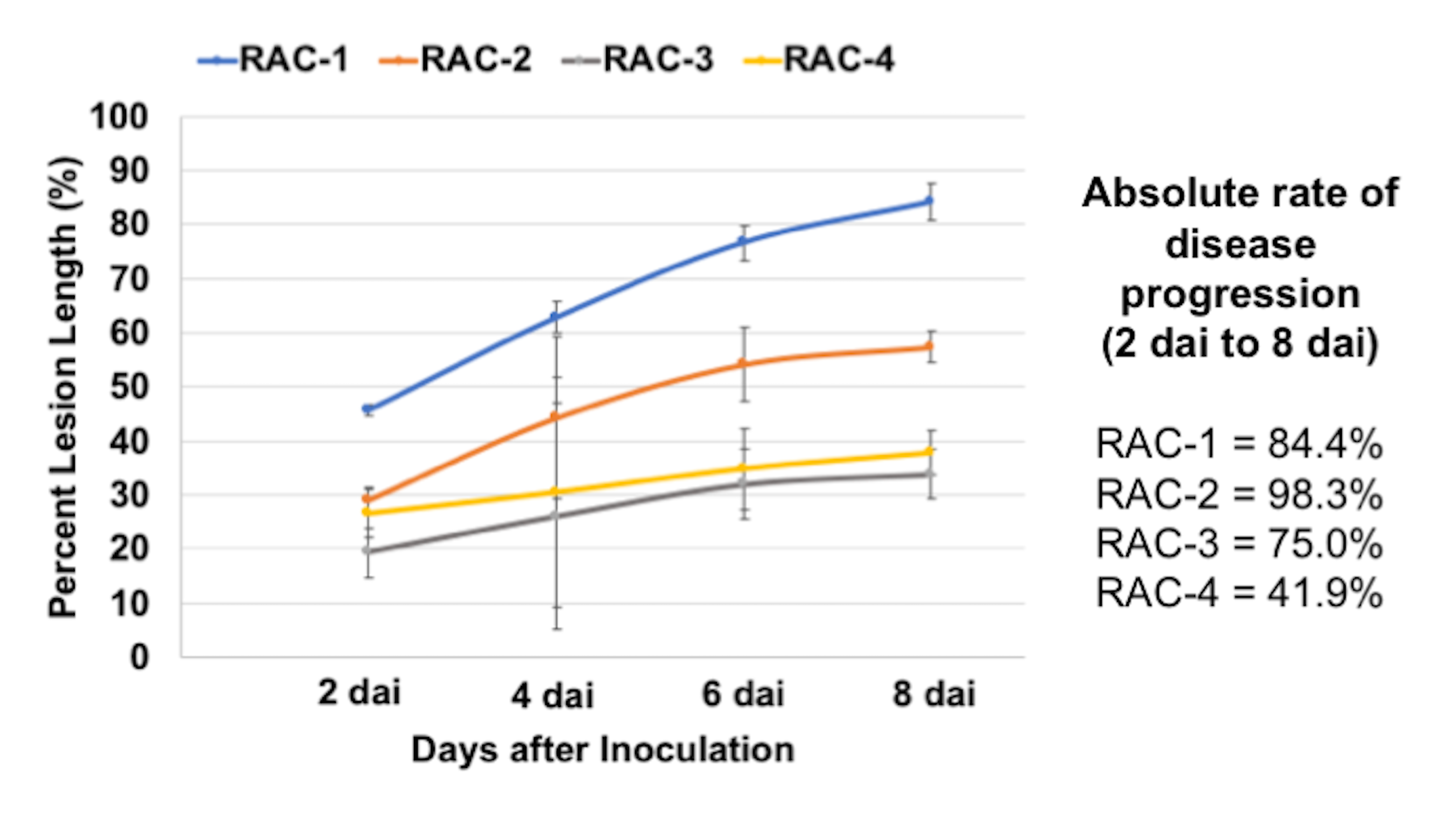
All inoculated young trees were evaluated 8 days after inoculation (dai) for fire blight infection, and for root traits. For both experiments, total shoot length, total leaf length, and length of necrosis of a leaf were measured in ‘cm’ using a ruler. The percent leaf lesion length (%) was calculated as the ratio of necrotic lesion length of a leaf to total leaf length multiplied by 100. Furthermore, chlorophyll contents of control and infected leaves were measured using a SPAD 502 Plus Chlorophyll Meter (Spectrum Technologies, Aurora, IL, USA). Average roots per node (count) and root dry mass (g) were simultaneously evaluated for all inoculated young trees (control and fire blight treated). Average roots per node were calculated by dividing total number of roots by number of nodes of a rootstock cutting used. At the end of each experiment at 8 dai, roots were shaved off each of the rootstocks, and dried in an oven to determine dry root mass.
For the second experiment, additional root trait data were digitally collected both at the beginning and at the end of the experiment. The root system from each ‘M.7’ rootstock was photographed by rotating it 360 degrees to capture the three-dimensional root surface area using a Canon EOS Rebel T5 Digital SLR camera (Cannon USA Inc., Melville, NY, USA). All raw images were first converted into greyscales, and then followed by binary conversion using the software ImageJ (https://imagej.nih.gov/ij/). Binary images were used to calculate the total root surface area (cm2) at the beginning of the experiment. Rootstocks were categorized into four different RACs, from lowest to highest root surface area (cm2). At the end of the experiment, roots were carefully dug out, and washed using a detergent and water. Roots were then spread on a flat surface, and photographed using a Canon EOS Rebel T5 Digital SLR camera. Photo-images were processed using an ImageJ software to calculate pre- and post-experiment root surface areas (cm2). Based on digital root diameter classifications, the root system of each young tree was separated into coarse (diameter > 1 mm) and fine (diameter < 1 mm) roots, dried in an oven, and then used to determine fine root dry mass (g), coarse root dry mass (g), and total root dry mass (g).
Statistical Analysis
All data collected for root and shoot traits, as well as for fire blight disease severity were used for statistical analysis. To test the relationships between root dry mass (g) and percent lesion length (%), the genotypes were grouped into three categories based on percent lesion length as Resistant (0-20% average PLL), Intermediate (21-80% average PLL), and Susceptible (81-100% average PLL). The data was tested for normality using Shapiro-Wilk test in R statistical software (http://www.R-project.org/) and log transformation was used to normalize the non-normal data. The normalized data was subjected to analysis of variance (ANOVA) using an R statistical software (http://www.R-project.org/). In addition, we also performed Kruskal-Wallis test using the original non-normal dataset to observe the significant differences. Mean values were compared using Tukey’s multiple comparison test. Broad-sense heritability (H2) was estimated as ratio of VG/VP, where VP corresponded to the total phenotypic variance explained by the genetic component variance (VG). The absolute rate of disease progression was calculated as the difference in PLL between day 8 and day 2, divided by PLL at day 2.
Average trait values were used to calculate Pearson correlation coefficients, as well as to perform hierarchical clustering with the “hclust” function and a principal component analysis (PCA) using “prcomp” function in R (http://www.R-project.org/). Hierarchical clustering estimated individual relationships based on extent of similarities between them; whereas, PCA utilized variance components to determine such relationships. Trait mean values were scaled to conduct both hierarchical clustering and PCA analysis. For hierarchical clustering, scaled trait datasets were used to generate a Euclidean distance matrix for estimation of inter-cluster distance with Ward’s linkage method. PCA analysis was conducted to obtain principal component (PC) eigenvalues and rotations to estimate contributions of different traits to explain variation by each PC. A PCA biplot was generated using the first two principal components (PC1 and PC2) to determine the overall genotypic variation and effects of root dry mass (g) on disease severity.
Leaf Sample Harvesting, RNA Extraction, 3’RNAseq Assay and Sequencing
Leaf tissues from M.7 rootstocks of contrasting initial root surface areas (cm2), in the second experiment, were used for RNA extraction and for gene expression analysis. Leaves were collected at 4 and 8 dai from two biological replicates of control and three biological replicates of bacterial-inoculated young trees of two contrasting RACs as described earlier [38, 57]. Leaf tissues were immediately immersed in liquid nitrogen, and stored at -800C until used for RNA extraction.
A SpectrumTM Plant Total RNA Kit (Sigma-Aldrich, St. Louis, MO, USA) was used to extract total RNA as per manufacturer’s protocol. Leaf tissues were ground into fine powder in liquid nitrogen, and 100 mg of leaf powder was transferred to 500 µl of lysis solution containing 2% b-mercaptaethanol. Samples were thoroughly mixed, placed at 56°C for 5 min, and centrifuged for 1 min at 13,000 rpm. The supernatant was passed through a filtration column at 13,000 rpm for 1 min to remove debris. The cleared lysate was mixed with 250 µl binding solution, and centrifuged through a binding column for 1 min at 13,000 rpm. After RNA binding, samples were washed twice using 500 µl wash solution I, as per manufacturer’s recommendations. Columns were centrifuged at maximum speed for 1 min during various washing steps. Dry columns were transferred to a new 2 ml centrifuge tube, and 50 µl elution buffer was added into the center of each binding column. Samples were kept in an elution buffer for 1 min, centrifuged at a maximum speed for 30 sec to elute RNA, and then this was repeated using 30 µl of elution buffer to increase RNA yield. The amount of RNA was determined using a NanoDropTM Spectrophotometer (Thermo Fisher Scientific, Grand Island, NY, USA), and the quality of RNA samples was assessed by running a 1% bleach agarose gel.
A total of 20 libraries were constructed and sequenced for RNA samples from control and bacterial-inoculated samples at the Genomics Facility at Cornell University (Ithaca, NY, USA). Briefly, 3’RNAseq libraries were prepared from ~500 ng of total RNA per sample using the Lexogen QuantSeq 3’ mRNA-Seq Library Prep Kit FWD for Illumina (https://www.lexogen.com/quantseq-3mrna-sequencing/). Libraries were quantified on a Molecular Devices Spectra Max M2 plate reader (with the intercalating dye QuantiFluor), and pooled accordingly for maximum evenness. The pooled sample was quantified by digital PCR, and sequenced along a single lane of an Illumina NextSeq500 sequencer to obtain single-end 1x86 bp sequences. Pooled libraries were de-multiplexed based upon six-base i7 indices using an Illumina bcl2fastq2 software (version 2.17; Illumina, Inc., San Diego, CA, USA).
Sequencing Data Processing and Analysis
A Trimmomatic (version 0.36) [58] software was used to remove Illumina adapters from de-multiplexed fastq sequences, as well as to remove low-quality reads for further analysis. Poly-A tails and poly-G stretches of at least 10 bases in length were then removed using the BBDuk program in the package BBMap (https://sourceforge.net/projects/bbmap/), but keeping reads of at least 18 bases in length after trimming. Often, poly-G stretches are obtained from sequencing past ends of short fragments (G = no signal).
Trimmed reads were then aligned to the GDDH13 Version 1.1 apple genome assembly (https://iris.angers.inra.fr/gddh13/downloads/GDDH13_1-1_formatted.fasta.bz2) using the STAR aligner (version 2.5.3a) [59]. For the STAR indexing step, the gff3 annotation file (https://iris.angers.inra.fr/gddh13/downloads/gene_models_20170612.gff3.bz2) was converted into a gtf format the gffread program from cufflinks (version 2.2.1) [60]. Key parameters used in the STAR indexing step (--runMode genomeGenerate) include --genomeChrBinNbits 18 and --sjdbOverhang 100. The STAR alignment step used the following key parameters: --outReadsUnmapped Fastx,
--outFilterMultimapNmax 10, --outFilterMismatchNoverLmax 0.06, --outSAMmode Full, --outSAMattributes Standard, --outFilterIntronMotifs, and RemoveNoncanonicalUnannotated. Output SAM files were converted to BAM using SAMtools (version 1.6) [61], and numbers of reads overlapping each gene in the gff3 file along the forward strand were counted using a HTSeq-count (version 0.6.1) [62]. A gene was deemed to be expressed using a criterion of detecting a minimum of five aligned high-quality read sequences against a particular gene model.
Gene Expression and Enrichment Analysis
The R package DESeq2 (version 1.20.0) [63] was used to obtain normalized counts from raw read counts. These counts were then used to conduct PCA of the 500 most variably-expressed genes following count normalization and variance stabilizing transformation, as well as for differential gene expression analysis. Control and bacterial-inoculated samples of each root class and time points were compared by deeming root class, time point, and inoculation treatment as distinct factors. The “contrast” function in DESeq2 was used to obtain expression analysis output for each comparison. For each gene, statistical significance of differential expression was based on a Wald test for a non-zero log fold change (LFC) estimate obtained from fitting a negative binomial generalized linear model [63]. Adjustment of p-values for multiple testing followed the Benjamini and Hochberg method [64]. Genes were deemed differentially expressed based on a log2Fold change threshold of 1.5 and a p-value of less than 0.01. All upregulated genes were determined based on positive log2Fold change values, and vice-versa.
Sets of differentially expressed genes from individual comparisons were used to perform a gene ontology (GO) term enrichment analysis using Fisher’s exact test with agriGO v2.0 [65]. Differentially expressed (DE) genes were compared to the complete set of fully-annotated genes in the GDDH13 Version 1.1 apple genome assembly. Estimated p-values were corrected using the Hochberg false discovery rate (FDR) correction method in agriGO v2.0. A p-value cutoff of less than 0.05 was used to determine significantly enriched GO terms.
Gene Co-expression Network Analysis
A co-expression network analysis of DE genes was performed using the weighted co-expression network analysis (WGCNA) package in R [66] to obtain modules of genes having similar expression patterns. A list of unique DE genes from each comparison was established by removing redundant genes from various differential gene expression analyses. Subsequently, normalized gene expression values for these unique DEGs were extracted to perform a co-expression network analysis. Co-expressed gene modules were then built using a single-step network generation and a module detection approach in WGCNA. Specifically, a network was generated by connecting all expression values in a dataset followed by detection of modules exhibiting very similar patterns of gene expression. A threshold value for module assignments was estimated using an unsigned topological overlap matrix (TOM); whereas, networks were constructed using a threshold power of 16, branch cut height of 0.25, and a minimum module size of 30. These co-expression modules were then visualized in Cytoscape v3.7.1 [67], and those highly connected genes, within each module, were identified using cytoHubba plugin [68] in Cytoscape. These modules were exported from WGCNA using a threshold of 0.2, and the top 20 highly connected genes were identified using four different algorithms including MCC, MNC, Degree, and EPC, implemented in cytoHubba. Finally, outputs were compared to select those hub genes that were consistently detected from all the four algorithms.