Single-sample landscape entropy (SLE) algorithm
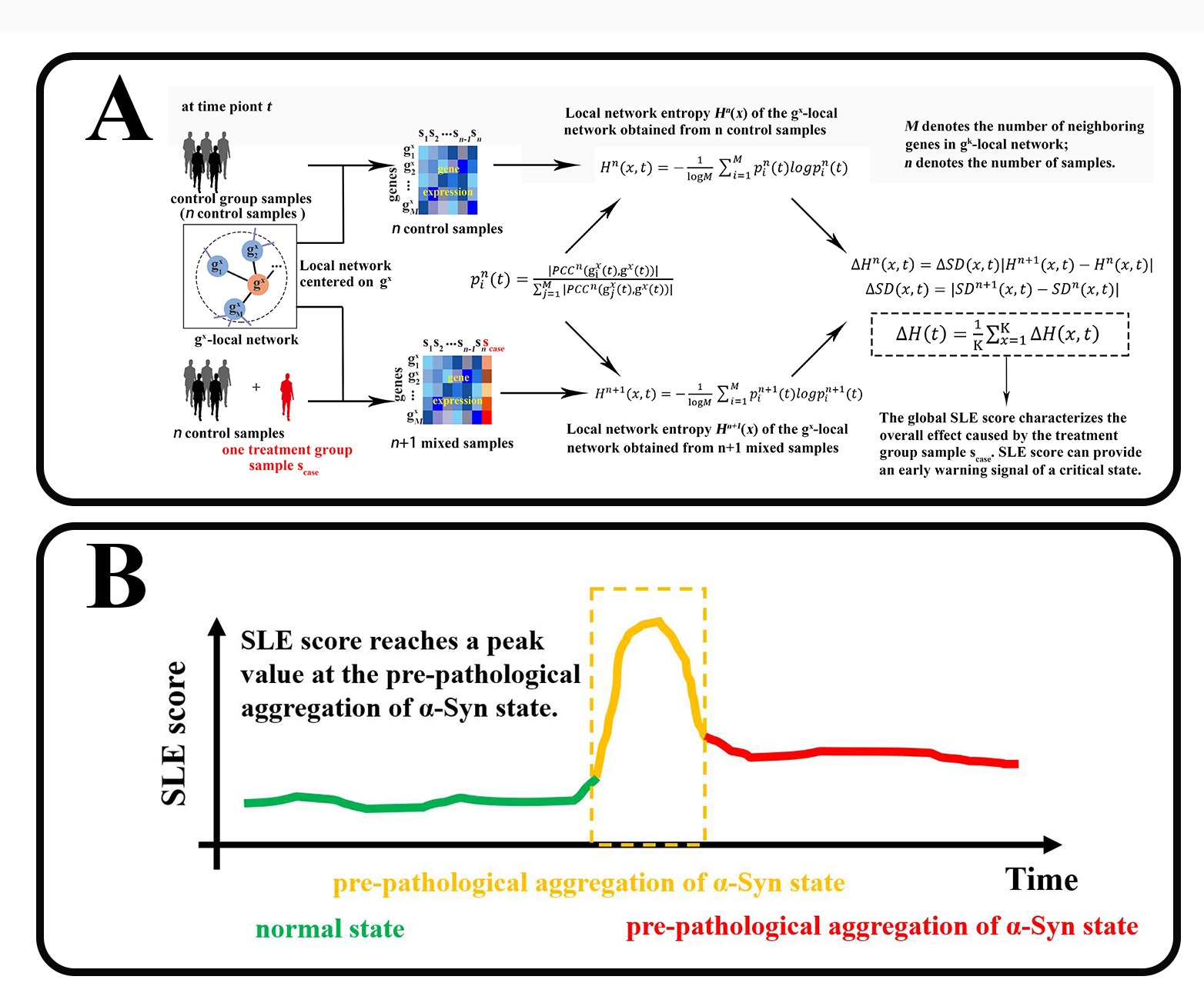
The SLE is a specific algorithm based on DNB method theory.26 It is used to explore dynamic differences between normal and predisease states and for identifying local network-based entropy, producing an SLE score that characterizes the statistical perturbations attributed by each treatment group sample to a given set of control group samples. Specifically, the SLE requires that a number of control group samples are first defined, and then, the following steps are performed:
[step 1] Use the STRING database to map genes to protein‒protein interaction (PPI) networks (or other template networks) to form the global network NG.
[step 2] Extract each local network from the global network NG such that each local network NX (X = 1, 2, 3, ..., K) is centred on the gene \({\text{g}}^{x}\). Suppose that there are M first-order neighbouring genes of gene \({\text{g}}^{x}\) in the \({\text{g}}^{x}\)-local network, that is, \({\text{g}}^{1x}\), \({\text{g}}^{2x}\), \({\text{g}}^{3x}\), …, \({\text{g}}^{Mx}\). If there are K genes in the global network NG, then there is a total of K local networks.
[step 3] For each local network NX (X = 1, 2, 3, ..., K) at time point t, based on n control samples {\({s}_{1}\left(t\right)\),\({s}_{2}\left(t\right)\)༌…༌\({s}_{n}\left(t\right)\)}, calc, l, te the local network entropy\({H}^{n}(x,t)\); i.e.,
$${H}^{n}(x,t)=-\frac{1}{\text{l}\text{o}\text{g}M}{\sum }_{i=1}^{M}{p}_{i}^{n}\left(t\right)log{p}_{i}^{n}\left(t\right)$$
1
with
$${p}_{i}^{n}\left(t\right)=\frac{\left|{PCC}^{n}\right({\text{g}}_{i}^{x}\left(t\right),{\text{g}}^{x}\left(t\right)\left)\right|}{\sum _{j=1}^{M}\left|{PCC}^{n}\right({\text{g}}_{j}^{x}\left(t\right),{\text{g}}^{x}\left(t\right)\left)\right|}$$
2
where \({PCC}^{n}\left({\text{g}}_{i}^{x}\right(t),{\text{g}}^{{x}}(t\left)\right)\) represents Pearson’s correlation coefficient for the central gene \({\text{g}}^{x}\) and a neighbouring gene \({\text{g}}_{i}^{x}\) based on n control samples. In Eq. (1), the superscript x indicates that the local network is centred at \({\text{g}}^{x}\), the subscript n denotes the number of samples and the constant M represents the number of neighbouring genes in the local network NX. In Eq. (2), The symbols \({\text{g}}^{x}\left(t\right)\) and \({\text{g}}_{i}^{x}\left(t\right)\) represent the expression of genes \({\text{g}}^{x}\) and \({\text{g}}_{i}^{x}\) at time point t, respectively.
[step 4] The newly added sample \({s}_{case}\left(t\right)\), which is a treatment group individual, is mixed with n control group samples. Based on n + 1 mixed samples {\({s}_{1}\left(t\right)\),\({s}_{2}\left(t\right)\)༌…༌\({s}_{n}\left(t\right)\)༌\({s}_{case}\left(t\right)\)}, calcu, ate t, e, local, network entropy \({H}^{n+1}(x,t)\); i.e.,
$${H}^{n+1}(x,t)=-\frac{1}{\text{l}\text{o}\text{g}M}{\sum }_{i=1}^{M}{p}_{i}^{n+1}\left(t\right)log{p}_{i}^{n+1}\left(t\right)$$
3
In Eq. (3), the definition of \({p}_{i}^{n+1}\) is similar to that in Eq. (2), but in Eq. (3) the correlation \({PCC}^{n+1}\left({\text{g}}_{\text{i}}^{x}\right(t),{\text{g}}^{x}(t\left)\right)\) is based on n + 1 mixed samples.
[step 5] Calculate the differential entropy \(\varDelta {H}^{n}(x,t)\) between \({H}^{n}(x,t)\) and \({H}^{n+1}(x,t)\); i.e.,
$$\varDelta {H}^{n}\left(x,t\right)=\varDelta SD(x,t)\left|{H}^{n+1}\right(x,t)-{H}^{n}(x,t\left)\right|$$
4
with
$$\varDelta SD(x,t)=\left|{SD}^{n+1}\right(x,t)-{SD}^{n}(x,t\left)\right|$$
5
where \({SD}^{n}\left(x,t\right)\) and \({SD}^{n+1}(x,t)\) are the standard deviations of the expression of the centre gene \({\text{g}}^{x}\) based on n control samples {\({s}_{1}\left(t\right)\),\({s}_{2}\left(t\right)\)༌…༌\({s}_{n}\left(t\right)\)} and n + 1 mixed sam, les {\({s}_{1}\left(t\right)\), \({s}_{2}\left(t\right)\)༌, ༌\({s}_{n}\left(t\right)\)༌\({s}_{case}\left(t\right)\)}, respectively. The differential, entro, y, \(\varDelta {H}^{n}(x,t)\) betw, en \({H}^{n}(x,t)\) and \({H}^{n+1}(x,t)\) represents differences caused by the newly added sample \({s}_{case}\left(t\right)\) from the treatment group. In other words, the local entropy \({H}^{n}\left(x,t\right)\) based on n control samples {\({s}_{1}\left(t\right)\)༌\({s}_{2}\left(t\right)\)༌…༌\({s}_{n}\left(t\right)\)}, \({H}^{n+1}(x,t)\) is compared with that based on n+1 mixed samples {\({s}_{1}\left(t\right)\)༌\({s}_{2}\left(t\right)\)༌…༌\({s}_{n}\left(t\right)\)༌\({s}_{case}\left(t\right)\)}, which indicates the perturbation, cause,, y the addition of single sample \({s}_{case}\left(t\right)\) to local network NX. In addition, to acc, unt f, r, gene, xpression fluctuations, the differential standard deviation \(\varDelta SD(x,t)\) is regarded as the weight coefficient.
[step 6] Calculate the weighted sum of \(\varDelta H\left(x\right)\) for all local networks; i.e.,
$$\varDelta H\left(t\right)=\frac{1}{K}{\sum }_{x=1}^{K}\varDelta H\left(x,t\right)$$
6
where constant K is the number of all genes. In Eq. (6), \(\varDelta H\left(t\right)\) indicates the overall effect caused by the addition of the treatment group sample \({s}_{case}\left(t\right)\) and is therefore referred to as the global SLE score, hereafter the SLE score, of the global network NG. Similarly, \(\varDelta {H}^{n}\left(x,t\right)\) in Eq. (4) is the local SLE score of the local network NX, which is centred on gene \({\text{g}}^{x}\).
When the system approaches the vicinity of the critical point, the DNB biomolecules exhibit significant collective fluctuations. In a local network with DNB biomolecules represented as nodes, Pearson’s correlation coefficients \({PCC}^{n+1}\left({\text{g}}_{\text{i}}^{x}\right(t),{\text{g}}^{x}(t\left)\right)\) becomes more similar or are equalized when the system is in a critical state, resulting in an increase in the local SLE score \(\varDelta H\left(x\right)\) in Eq. (4). In addition, \(\varDelta SD(x,t)\) in Eq. (6) increases accordingly, which contributes to the increase in the global SLE score \(\varDelta H\left(t\right)\). Therefore, the SLE score can provide an early warning signal of an impending critical state transition. When the global SLE score \(\varDelta H\left(t\right)\) reaches a peak value at a certain time point, the time point is considered to be indicative of the critical state (Supplementary Fig. 1).
The GEO database
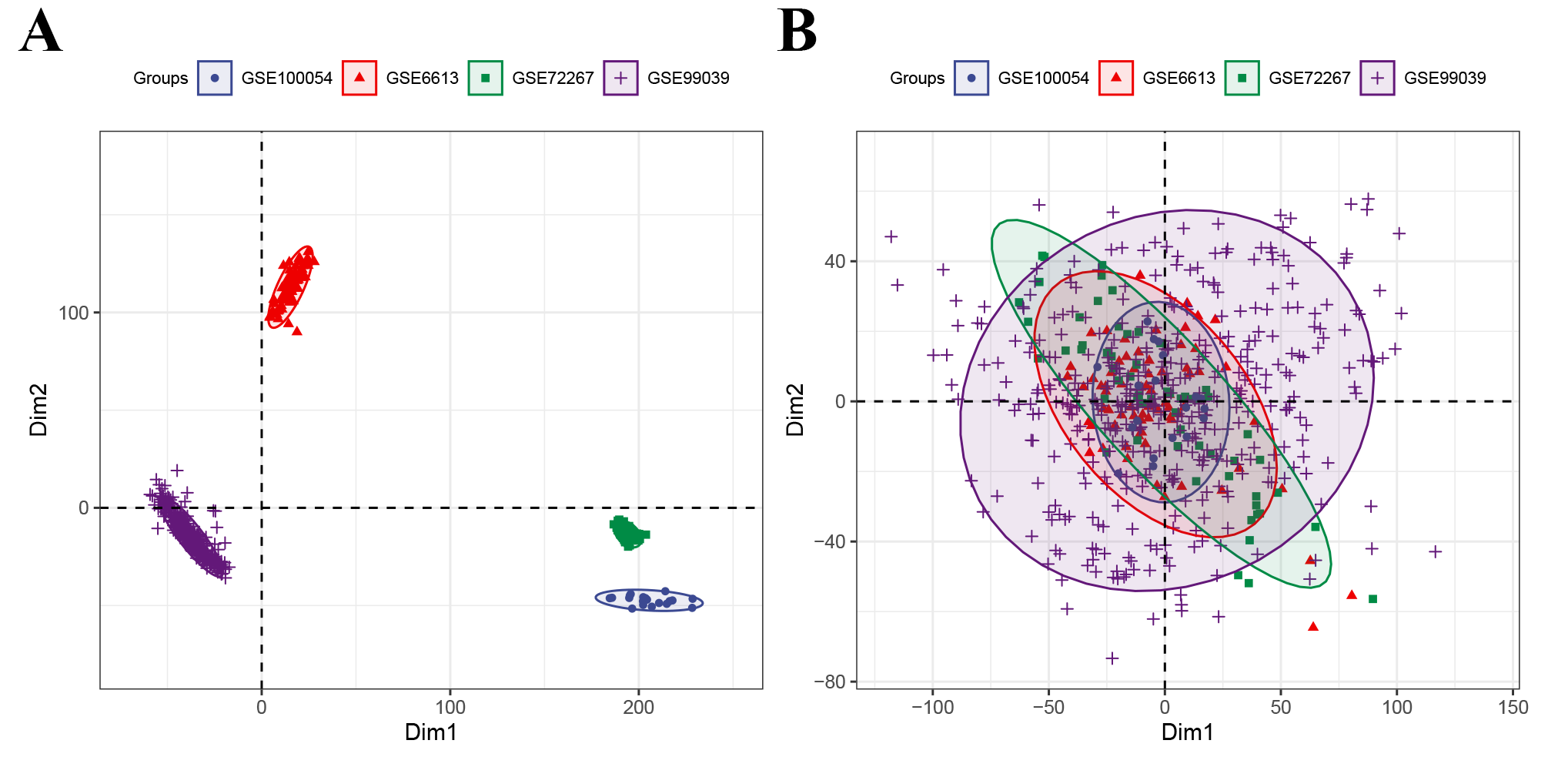
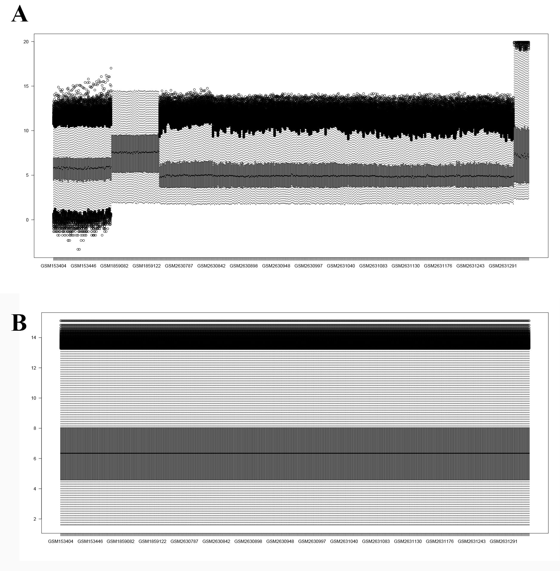
We searched a blood microarray dataset in the GEO database using the keywords “PD,” “blood,” and “Homo sapiens” and ultimately selected the GSE6613, GSE72267, GSE99039 and GSE100054 databases, which included information on 305 PD patients and 283 healthy controls (HCs) in total. Detailed information on the datasets is provided in Supplementary Tables 6 and 9. We downloaded the raw data and platform information of these datasets and then annotated the probe ID after preprocessing the raw data. The common genes were merged into three expression matrices, and the batch effect among them was removed. The raw data of these datasets were processed through the affy package to read the .cel file and RMA algorithm for background correction and data normalization. Then, we normalized three gene expression matrices, and the interbatch difference was removed using the removebatcheffect function of the limma package. The boxplots and two-dimensional PCA plots before and after removing the batch effect are shown in the Supplementary Figures. After normalization, the median expression values of the samples from the three datasets were at the same level, and the PCA plot showed that the difference among them was decreased, indicating that the merged expression matrix was appropriate for use in further analysis.
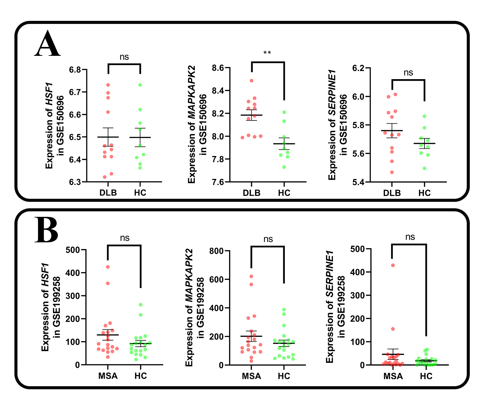
We then collected two PD transcriptome datasets consisting of brain sample data in the GEO database: the GSE20292 dataset (with 11 PD patients and 18 HCs) and the GSE68719 (with 29 PD patients and 44 HCs). The GSE20292 dataset samples, sequenced using the Affymetrix Human Genome U133 Array platform, had been obtained from the substantia nigra in the brain. The GSE68719 dataset samples, sequenced using the Illumina HiSeq 2000 platform, were obtained postmortem from the prefrontal cortex area (BA9). Furthermore, we collected two transcriptome datasets with information on other α-Syn-associated diseases in the GEO database: the GSE150696 dataset (12 dementia with Lewy bodies (DLB) patients and 9 HCs) and the GSE199258 dataset (with 19 multiple system atrophy patients and 19 HCs). The GSE150696 dataset samples, sequenced using the Affymetrix Human Transcriptome Array 2.0 platform, were obtained postmortem from the prefrontal cortex area (BA9). The GSE199258 dataset samples, sequenced using the Illumina HiSeq 2500 platform, were obtained from peripheral blood.