Instead than being driven by aerodynamic concerns, new generations of tall structures are becoming taller, more flexible, and slimmer due to architectural factors, functional requirements, and site constraints. Tall buildings are hence more vulnerable to lateral loads like wind. Aerodynamic form adjustment can considerably lessen these effects. In terms of fluid dynamics, drag force describes how a solid object behaves in the direction of the relative wind flow velocity. This investigation involves drag coefficient of aerodynamically shape modified buildings with combinations such as setback with void(S + V), corner cut with void(CC + V), setback with corner cut(S + CC) comparatively with square, setback and corner cut. The model is generated using SOLIDWORKS software and further analyse in the ANSYS FLUENT 19.2.) The velocity and pressure contours for these model has been studied along with drag and lift coefficient.
Research Article
Reducing Impact of Wind on Tall Buildings Through Aero-dynamic Shape Modifications
https://doi.org/10.21203/rs.3.rs-2082175/v1
This work is licensed under a CC BY 4.0 License
Version 1
posted
You are reading this latest preprint version
CFD
SolidWork
Wind load
Aerodynamic shape modification
A new generation of tall, slender, and light buildings have been developed as a result of the development of high strength materials, improved structural behaviour understanding, sophisticated analytical tools, and structural design techniques. In addition to gravity stresses, these structures are also vulnerable to time-varying loads from wind, earthquakes, etc. Over specific frequency ranges, these loads are dominating. One of the most important factors in the design of buildings is the wind loadsEmploying "Aerodynamic Shape Modification" techniques is one way to lessen the wind pressures on buildings. These techniques successfully alter the aerodynamic shape of the buildings to lessen wind loads. They do this by utilising straightforward and creative design characteristics. Aerodynamic changes help by preventing strong corner vortices from forming, rupturing coherent vortex formations, or rerouting flows in the separation zone over the roof edge or away from the weak components.
1.1 WIND
In most cases, the wind blows quickly and horizontally toward the ground. High rise structures are therefore more vulnerable to wind loads and wind-induced excitations, which could decrease their structural safety and be uncomfortable for the occupants. Also, the cost of the structure may rise as a result of these excessive motions' high base loads. For typical tall buildings, the aerodynamic forces are the torsional moment, the lift force, and the drag force (following the wind) (Fig. 1). According to Fig. 1, wind vortex shedding causes dynamic across-wind loading, which typically dominates the wind-induced response of tall buildings.
A.G. Davenport (1961a) proposed that the statistical ideas of the stationary time series are employed to ascertain how a straightforward construction will react to a turbulent, gusty wind. This makes it possible to explain concepts like peak stresses, accelerations, deflections, etc. in terms of the mean wind speed, the gustiness spectrum, and the mechanical and aerodynamic characteristics of the structure. A. G. Davenport (1963b) found the involution of a satisfactory to the loading of structures by gusts. It is suggested that a statistical approach based on the concepts of the stationary random series appears to offer a promising solution. A. G. Davenport (1967) developed the "Gust Factor Approach" for analytical prediction of along wind response of tall buildings.
1.2 AERODYNAMIC MODIFICATIONS TO BUILDING SHAPE
The largest wave of tall building construction in history is currently taking place throughout the world. The weight, stiffness, and damping values of tall structures have been decreased by the use of lighter floors, greater strength materials, and curtain wall systems. Tall buildings are therefore more vulnerable to wind loads.Based on geometry, there are many atypical tall buildings are as follows:
1. Basic
1.1. Square
1.2. Rectangle
1.3. Circle
1.4. Triangle
2. Corner modification
3. Void/Opening
4. Tapered
5. Setback
6. Helical
7. Tilted
8. Combinations
The current work examines the CFD analysis of a square-shaped structure that has undergone several aerodynamic alterations. The study is conducted for modifications like setback, corner cut, void\opening and their combinations such as corner cut with opening, setback with corner cut, setback with void\opening.
2.1 MODELLING
The analysis work in this paper is based on the outcomes of CFD simulations. SolidWorks was used to produce the building's 3D models, as seen in the square model in Fig. 2.2.1. For this study's tunnel modelling, ANSYS Design Modeler is utilized. The simulation of wind tunnel testing was done with ANSYS FLUENT. The drag coefficients of the building were calculated using these simulated wind loads.
2.2 MODEL
According to Fig. 2.2.2, the model employed in the study has a square-shaped plan. The building has a B/H ratio of 1/8, with a breadth of 50 m and a height of 400 m. To make it easier for further wind tunnel experiments, the model has been scaled down to a 1:1000 scale. The models of the building were made with three aerodynamic modifications including setback, corner cut, void\opening and their combinations such as corner cut with opening, setback with corner cut, setback with void\opening as shown in Fig. 2.2.2.
2.3 DETAILS OF COMPUTATIONAL DOMAIN
According to Fig. 2.3, the wind tunnel is a rectangular box. It is designed to have a downstream fetch of 15B and an upstream fetch, side clearance, and height of 5B, where H is the height of the building. These domain dimensions were determined by Y. Meng and K. Hibi[13]. In order to prevent the recommended inflow profiles along the empty computational domain of the building's windward side from deteriorating, the windward distance was set only a little bit below the suggestions by the AIJ guideline [14].
Both the domain's inlet and output have a velocity inlet and an outflow condition applied as their respective boundary conditions. Zero Pa is assumed to be the outlet's relative pressure. The building's walls are given a no-slip wall condition, while the free slip wall condition is applied to the domain's other four rectangular sides.
2.4 BOUNDARY CONDITIONS AND NUMERICAL METHODS
The wind environment in this study is produced using the well-known k-epsilon (k-) Reynold's-averaged Navier-Stokes turbulence model. The variance of velocity fluctuations is known as the turbulent kinetic energy, or k. The turbulence eddy dissipation, or, calculates the rate at which velocity fluctuations dissipate. The turbulence kinetic energy and turbulence dissipation rate's differential transport equations provide the values for k and ɛ.

The fluid's density and velocity are represented by ρ and U, respectively. Pk is the kinetic energy of the generated turbulence that results from mean velocity gradients, Pb is the generation that results from buoyancy, and YM is the contribution of fluctuation dilatation incompressible turbulence to the overall dissipation rate. C1 and C2 are constants. Prandtl number for k and ε are σk and σε. The values of C1ε, σk and σε are 1.44, 1 and 1.3. Atmospheric boundary layer (ABL) wind profile is used, is governed by the power law equation, which is given as follows:

yref is the height of the computational domain, uref is the free stream velocity, and the power law coefficient is 0.27, where u is the velocity at heights above ground,(for sub-urban area).
2.5 VALIDATION OF WIND PROFILE
To confirm the accuracy of the work, the velocity profile that was developed must be evaluated. The wind tunnel data utilized as illustrated in Fig. 5 and the computed profile are compared. Since the wind environments employed in both situations are similar, Fig. 2.5 demonstrates that the simulated profile reflects the profiles from wind tunnel studies and the power law equation with sufficient accuracy. As a result, it may be said that the study's flow characteristics are acceptable.
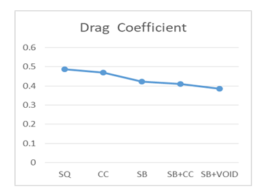
The square Model is used for validation purpose. The result obtained like Drag coefficient values are 0.48. The corresponding value obtained from this study are in close range as compare with Yukio Tamura, Hideyuki Tanaka, Kazuo Ohtake, Masayoshi Nakai, Yongchul Kim [2010].
2.6 MESHING
The software ANSYS FLUENT is used for meshing. To ensure that the solution variables decrease to acceptable values, mesh is modified. Tetrahedron meshing is applied. The domain face and edge has been appropriately adjusted. Figure 2.6 illustrates the meshing of the base model. For each model, grid convergence studies were done. To obtain convergent values of drag coefficients, the mesh conditions are modified while increasing the number of elements.
The outcomes of the CFD study performed on the models are described in the sections below. For each model, the values of the drag force coefficients are examined. The pressure contours and velocity contours of the each model for are also be studied.

Where V is the mean wind speed, A is the plan area that the wind is blowing onto, and F is the drag force. The density of air is assumed to be 1.185 kg/m3.
The velocity contours is as follows:
The Pressure Contour from top view is as follows:
3.2 Conclusion
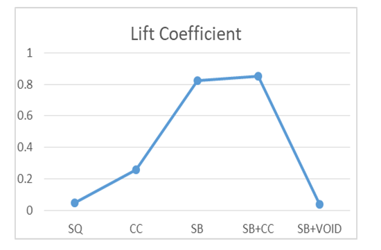
The drag coefficient values is maximum for square model and minimum for SB + Void Model. As certain modification is done on models such as CC, SB and SB + CC, the values are in between 0.5 to 0.3 as shown in chart1. Although the wind force coefficients for the SQ and SB + VOID model were the smallest among the models tested. The lift coefficient is small for SQ and SB + VOID and highest for SB + CC. The lift and drag coefficient are in the range of 0–1.
- M. Gu, Y. Quan, Across-wind loads of typical tall buildings, Journal of Wind Engineering and Industrial Aero- dynamics 92 (2004) 1147–1165.
- Y. L. Lo, X. Tian, Q.-S. K. F. Tee, Y.-G. Li, Li, Aerodynamic treatments for reduction of wind loads on high- rise buildings, Journal of Wind Engineering & Industrial Aerodynamics 172 (2018) 107–115
- Y.-G. Li, M.-Y. Zhang, Y. Li, Q.-S. Li, S.-J. Liu, Experimental study on wind load characteristics of high-rise buildings with the opening, John Wiley & Sons, Ltd, 2020 URL https://doi.org/10.1002/tal.1734.{\copyright}
- Y. Chul, Kim, J. Kanda, Characteristics of aerodynamic forces and pressures on square plan buildings with height variations, J. Wind Eng. Ind. Aerodyn 98 (2010) 449–465.
- Y. Chul, Kim, J. Kanda, Wind pressures on tapered and set-back tall buildings, Journal of Fluids and Structures 39 (2013) 306–321.
- Y. Tamura, H. Tanaka, K. Ohtake, M. Nakai, Y. Kim (2010) Aerodynamic Characteristics of Tall Building Models with Various Unconventional Configurations, 2010 Structures Congress © 2010 ASCE 3104-3113.
- Y. Tamura, H. Tanaka, K. Ohtake, M. Nakai, Y. Kim, Experimental investigation of aerodynamic forces and wind pressures acting on tall buildings with various unconventional configurations, J. Wind Eng. Ind. Aerodyn (2012) 179–191.
- . C. Kim, Y. Tamura, H. Tanaka, K. Ohtake, E. K. Bandi, A. Yoshida, Wind-induced responses of super-tall buildings with various atypical building shapes, J. Wind Eng. Ind. Aerodyn 133 (2014) 191–199.
- A. Elshaer, G. Bitsuamlak, Multiobjective Aerodynamic Optimization of Tall Building Openings for Wind-Induced Load Reduction, J. Struct. Eng 144 (10) (2018).
- C. Zheng, Y. Xie, M. Khan, Y. Wu, J. Liu, Aero- dynamic treatments for reduction of wind loads on high- rise buildings, Journal of Wind Engineering & Industrial Aerodynamics 172 (2018) 107–115.
- M. S. Thordal, J. C. Bennetsen, S. Capra, A. K. Kragh, H. Holger, H. Koss, Towards a standard CFD setup for wind load assessment of high-rise buildings: Part 2 - Blind test of chamfered and rounded corner high-rise buildings, Journal of Wind Engineering & Industrial Aerodynamics 205 (2020).
- Code of Practice for design loads for building and structures, Part-3 wind loads IS-875 (PART-3) 2015. Published by Bureau of Indian Standards.
- Y. Meng, K. Hibi, Turbulent measurements of the flow field around a high-rise building, J. Wind Eng. 76 (1998) 55e64.
- A. Mochida, Y. Tominaga, S. Murakami, R. Yoshie, T. Ishihara, R. Ооka, Comparison of various ke models and DSM applied to flow around a high-rise building-report on AIJ cooperative project for CFD prediction of wind environment, Wind Struct. 5 (2002) 227e244.
- Y. Tominaga, A. Mochida, R. Yoshie, H. Kataoka, T. Nozu, M. Yoshikawa, et al., AIJ guidelines for practical applications of CFD to pedestrian wind environment around buildings, J. Wind Eng. Ind. Aerodyn. 96 (2008) 1749.
Chart 1 and 2 is available in Supplementary Files section.
No competing interests reported.
- Chart1.png
Chart -1: Comparison of Drag coefficient

- Chart2.png
Chart -2: Comparison of Lift coefficient