A Country’s progress and development are mainly dependent on its indigenous energy supply capacity. For the past few decades, Pakistan is facing a severe energy crisis mainly due to political instability and a lack of renewable energy policies designed by the present as well as previous governments. According to Pakistan economic survey 2019-20, still, there is a shortfall of about 3000MW in the electrical sector for the summer of 2020. Wind speed models can be utilized for developing effective policies for the production of efficient renewable resources. In this study, power Burr X distribution was utilized as an alternative probabilistic model for the better evaluation of wind energy potential. The performance of the model is observed for wind speed data taken from different locations of Sindh province in Pakistan. The findings indicate that the power Burr X distribution is more preferable for the evaluation of wind speed potential as compared to Weibull and other wind speed distributions.
Research Article
Use of Power Burr X Distribution in the Analysis of Wind Speed for Certain Regions of Pakistan
https://doi.org/10.21203/rs.3.rs-2083233/v1
This work is licensed under a CC BY 4.0 License
Version 1
posted
You are reading this latest preprint version
Renewable energy sources
power Burr X distribution
maximum likelihood estimation
power density error
wind speed modelling
Improvement in technology and increase in population demand caused an enormous use of energy worldwide. One of the key elements for the development of a country is the production of energy (Akgül et al. 2016). Despite rich gas and coal reserves, Pakistan is still facing serious energy crisis due to huge shortfall between the production and consumption of energy (Ahmed et al. 2010). To fulfill energy demand, usually countries rely on the conventional resources such as fossil fuels. However, these sources are not preferable mainly due to their contribution in environmental degradation, such as substantial carbon dioxide emission, ozone depletion, escalation of air pollution, which is eventually causing global warming and climate change (Bilir et al. 2015).
The world is therefore, looking for environment friendly options to fulfill their energy needs, such as renewable energy resources, which includes solar, geothermal, and wind. The most dominant, rapid creation and extensively utilized wellspring of the sustainable power source is wind energy which is perfect and practical for the ecosystem (see e.g. Alavi et al. 2016). Therefore, more than 90 countries have wind farms to fulfill their energy demands, and 9 of them have more than 10GW installed capacity (Dupré et al. 2020). Half of the wind power capacity has been installed in the last five years and now developed countries such as European Union and the United States are focusing on this efficient source of energy (Solaun and Cerdá, 2020).
Generally, numerous factors are responsible for significant wind speed variations. These include climate, surface outline, ecological settings and landscapes. Due to complex variation of wind speed on a wind turbine, power extraction of wind speed demands cultured practices for optimization (Kitaneh et al. 2012). The economical and efficient gain of wind energy is based on two important factors. One of them is the preferable choice of geological location for installation of a wind farm and the other is the choice of best statistical model with low estimation cost for the identification of wind speed characteristics.
From last few decades, two parameters Weibull distribution is effectively practiced for the modeling of wind speed potential (Akdağ and Güler, 2015; Rocha et al. 2012; Akpinar and Akpinar, 2009). However, it has been explored in the literature that the generalized distributions can be used for efficient model fitting instead of Weibull distribution such as inverse Weibull (Akgül et al. 2016), generalized Lindley and power Lindley (Arslan et al. 2017), extended generalized Lindley (Kantar et al. 2018), inverse logistic (Chiodo et al. 2018), extreme value distribution (Sarkar et al. 2011), Gamma (Morgan et al. 2011), generalized Gamma (Mert and Karakuş, 2015), Burr XII (Usta, and Kantar, 2012), Johnson SB (Soukissian, 2013; Johnson et al. 1995).
Burr X (BX) distribution belongs to the system of twelve probabilistic models was proposed by Burr (1942). Numerous features of BX have been discussed by different authors (Ahmad, 1997; Surles and Padgett, 2001; Raqab and Kundu, 2006). The two-parameter BX distribution was proposed by Surles and Padgett (2005) and it is also known as generalized Rayleigh. As generalized Rayleigh distribution is a special case of generalized Weibull, therefore, BX distribution can be used as an alternate of Weibull and Rayleigh distribution for data modeling. However, the model has a significant role in the modeling of failure rate and induced significant attention for the modeling in numerous fields such as reliability analysis, hydrology, and medicines.
The main purpose of carrying out this study was to use power Burr X (PBX) distribution as an alternative of Weibull distribution for efficient wind speed analysis. The literature emphasizes that the Weibull may not be used for effective modeling of wind speed at a different location in the world. Therefore, we explored PBX distribution over Weibull and other well-known distributions for the evaluation of wind potential in Pakistan. The comparison of PBX was carried out with generalized Weibull (GW), Weibull (W), Lindley (Li), power Lindley (PLi), Power Lomax (PL), and Burr X (BX) distribution. The findings of this study can be used by government policymakers as well as private multinational agencies for better investment in renewable energy projects in Pakistan.
The PBX distribution with two shape parameters (unit less) and one scale parameter (ms− 1) was suggested (Usman and Ilyas, 2020). The cumulative distribution function \(G (\bullet )\) and density function \(g(\bullet )\) were given as,
$$G\left(z;a,b,\theta \right)={\left(1-{e}^{\left(-{\left(b{z}^{\theta }\right)}^{2}\right)}\right)}^{a-1} for z>0, a,b,\theta >0 \left(1\right)$$
$$g\left(z;a,b,\theta \right)=2a{b}^{2}\theta {z}^{2\theta -1}{e}^{\left(-{\left(b{z}^{\theta }\right)}^{2}\right)}{\left(1-{e}^{\left(-{\left(b{z}^{\theta }\right)}^{2}\right)}\right)}^{a-1} \left(2\right)$$
Here, \(a\) and \(\theta\) are positive shape parameters and \(b\) is scale parameter with unit (\(m{s}^{-1}\)). Burr X can be obtained from PBX distribution for \(\theta =1\), while significant rearrangement of parameters can make the model exponentiated Weibull. The PDF curves and hazard rate curves (HRC) for the PBX model are given in Fig. 1. However, the density and distribution function of participant models are defined in Table 1.
| Distribution | Density Function (PDF) | Distribution Function (CDF) |
|---|---|---|
| Generalized Weibull (GW) | \({g}_{GW}\left(z\right)=\frac{ab\theta }{{z}^{1-b}}{\left(1+\theta {z}^{b}\right)}^{a-1}{e}^{\left(1-{\left(1+\theta {z}^{b}\right)}^{a}\right)}\) | \({G}_{GW}\left(z\right)=1-{e}^{\left(1-{\left(1+\theta {z}^{b}\right)}^{a}\right)}\) |
| Power Lomax (PL) | \({g}_{PL}\left(z\right)=\frac{ab{\theta }^{a}{z}^{b-1}}{{\left(\theta +{z}^{b}\right)}^{a+1}}\) | \({G}_{PL}\left(z\right)=1-\frac{{\theta }^{a}}{{\left(\theta +{z}^{b}\right)}^{a}}\) |
| Power Lindley (PLi) | \({g}_{PLi}\left(z\right)=\frac{{a}^{2}b{z}^{b-1}}{a+1}\left(1+{z}^{b}\right){e}^{-a{z}^{b}}\) | \({G}_{PLi}\left(z\right)=1-\left(1+\frac{a{z}^{b}}{a+1}\right){e}^{-a{z}^{b}}\) |
| Burr X (BX) | \({g}_{BX}\left(z\right)=a{b}^{2}z{e}^{\left(-{\left(bz\right)}^{2}\right)}{\left(1-{e}^{\left(-{\left(bz\right)}^{2}\right)}\right)}^{a-1}\) | \({G}_{PLi}\left(z\right)={\left(1-{e}^{\left(-{\left(bz\right)}^{2}\right)}\right)}^{a}\) |
| Lindley (Li) | \({g}_{Li}\left(z\right)=\frac{{a}^{2}}{a+1}\left(1+z\right){e}^{-az}\) | \({G}_{Li}\left(z\right)=1-\left(1+\frac{az}{a+1}\right){e}^{-az}\) |
3.1 Wind Data Description
Data were collected from Pakistan Meteorological Department (PMD) from three different stations (Sanghar, Sujawal, and Umerkot) of Pakistan. A study conducted by Alam et al. (2011) indicated that wind energy can be increased by changing the hub-height from 50 to 60 meters. Therefore, the observations are being taken for the period 2017-18 at 60 meters height for a 10-minute average. The data is also available at https://energydata.info/dataset/pakistan-wind-measurement-data. Table 2 provided the geographical location, altitudes and the number of collected observations for all three stations.
| Stations | Geographical Locations | Altitude | Farm Height | Time-Interval | No. of Observations |
|---|---|---|---|---|---|
| Sanghar | \(26^\circ {02}^{{\prime }}{00}^{{\prime }{\prime }}N; 68^\circ 57{\prime }00{\prime }{\prime }E\) | 68.9 feet | 60 meters | 10 minute | 52474 |
| Sujawal | \(24^\circ {36}^{{\prime }}{23}^{{\prime }{\prime }}N; 68^\circ 04{\prime }19{\prime }{\prime }E\) | 19.0 feet | 60 meters | 10 minute | 48565 |
| Umerkot | \(25^\circ {22}^{{\prime }}{12}^{{\prime }{\prime }}N; 69^\circ 43{\prime }48{\prime }{\prime }E\) | 13.0 feet | 60 meters | 10 minute | 52127 |
3.2 Data Assessment
Efficient and economical model selection was carried out by familiar and consistent criteria. The study utilizes five reliable and extensively used statistical indicators to observe the best fit of the considered probability distributions used for wind speed analysis. The methods for these selection criteria are briefly discussed.
3.2.1 Akaike information criterion
An Akaike Information Criterion (AIC) is an important goodness-of-fit measure used for the model selection by estimating the quality of each model. However, it is also used to provide relative measures about lost information when the observed probability model is operated to illuminate certainty. It depends on the likelihood function obtained from the maximum likelihood estimators and the number of estimated parameters (Akaike, 1998).
$$AIC=2M-2\text{ln}\mathcal{l} \left(3\right)$$
Here, M is the number of estimated parameters while \(\mathcal{l}\) is the estimated log-likelihood value.
3.2.2 Kolmogorov-Smirnov test
The Kolmogorov-Smirnov (KS) goodness-of-fit test was suggested (Kolmogorov, 1933; Smirnov, 1939). It is a non-parametric test based on the extreme difference between an empirical CDF and hypothetical CDF of the continuous probability distribution. Mathematically,
$$KS=\underset{1\le k\le m}{\text{max}}\left|{\widehat{G}}_{k}-\frac{k}{m+1}\right| \left(4\right)$$
Here, \(\widehat{G}\) represents the theoretical CDF of the \(m\) ordered data points of the \({k}^{th}\) ordered observations.
3.2.3 Root mean square error (RMSE)
The RMSE is another goodness-of-fit criterion used in this study to classify the accuracy of the observed models. The measurement compares the actual probabilities and the expected probabilities. The value of RMSE is closer to 0 is considered as the better fitted model on comparison. RMSE is defined as
$$RMSE={\left(\frac{1}{m}\sum _{k=1}^{m}{\left({\widehat{G}}_{k}-\frac{k}{m+1}\right)}^{2}\right)}^{\frac{1}{2}} \left(5\right)$$
3.2.4 Coefficient of determination
The coefficient of determination \(\left({R}^{2}\right)\) for the observed distributions could be obtained from the methodology given in Eq. (6). The measurement utilized the probabilities from the CDF of the observed distribution and the expected probabilities. The close value of \({R}^{2}\) to one is considered as the better fit for the comparison. If \(\widehat{G}\left(\bullet \right)\) is the predicted cumulative probabilities for \(m\) number of observations and \(\stackrel{-}{\widehat{G}}\left(\bullet \right)\) is the average of expected CDF, then the \({R}^{2}\) is obtained as
$${R}^{2}=1-\frac{\sum _{k=1}^{m}{\left(\widehat{G}\left({Z}_{k}\right)-\frac{k}{m+1}\right)}^{2}}{\sum _{k=1}^{m}{\left(\widehat{G}\left({Z}_{k}\right)-\stackrel{-}{\widehat{G}}\left({Z}_{k}\right)\right)}^{2}} \left(6\right)$$
3.2.5 Chi-square goodness-of-fit test
Snedecor and Cochran (1967) had presented the chi-square \((Chi.sq)\) goodness of fit test to observe whether the sample data follow the population of the observed distribution. The test statistic for chi-square test is given in Eq. (7).
$$Chi.sq=\sum _{k=1}^{m}\frac{{\left({O}_{k}-{E}_{k}\right)}^{2}}{{E}_{k}} \left(7\right)$$
Here, \({O}_{k}\) represent the observed probabilities and \({E}_{k}\) represent the expected probability of the observed distribution function.
Before probabilistic analysis, some measures are given for initial description such as minimum, maximum, mean, variance, skewness, kurtosis and coefficient of variation for wind speed data for all stations.
|
Stations |
Min.\(\left(m{s}^{-1}\right)\) |
Max.\(\left(m{s}^{-1}\right)\) |
A.W.S\(\left(m{s}^{-1}\right)\) |
Variance |
Skewness |
Kurtosis |
C.V (%) |
|---|---|---|---|---|---|---|---|
|
Sanghar |
0.0010 |
20.6430 |
6.3100 |
9.1230 |
0.3074 |
2.7371 |
14.632 |
|
Sujawal |
0.0346 |
16.5699 |
6.9743 |
6.2615 |
0.0215 |
3.0295 |
15.101 |
|
Umerkot |
0.0126 |
16.9004 |
6.0967 |
7.5987 |
0.3802 |
2.9883 |
45.214 |
The average wind speed (A.W.S) for all observed stations is more than 6\(m{s}^{-1}\) while the observed maximum speed for all stations is more than 16\(m{s}^{-1}\). The calculated skewness for Sanghar, Sujawal and Umerkot stations is 0.3074, 0.0215 and 0.3802 respectively; therefore, all data sets are positively skewed. Moreover, variance, kurtosis and coefficient of variation (C.V) are expounded in Table 3 for all three stations.
It is known that the evidence related to failure rate can lead to an assortment of appropriate distribution. Therefore, we have utilized the total time on test (TTT) plots for the assessment of the failure rate. For constant failure rate, the TTT plot is diagonally straight. The convex shape of the TTT plots show decreasing failure rate while the concave shape of the TTT plots shows an increasing failure rate. Moreover, first convex and then concave shape TTT plots provide the bathtub behavior of failure rate. Since TTT plots are given in Fig. 2 for Sanghar, Sujawal and Umerkot stations show the concave shape thus all data sets contain increasing failure rate and the PBX distribution is appropriate for such kinds of data sets.
|
Stations |
Competitor Models |
|||||||
|
PBX |
GW |
PL |
W |
BX |
PLi |
Li |
||
|
Sanghar |
\(a\) |
0.68670 |
1.66970 |
19.4319 |
2.20922 |
1.13190 |
0.09995 |
0.28209 |
|
\(b\) |
0.05404 |
1.95430 |
2.24453 |
7.12206 |
0.14861 |
1.55014 |
- |
|
|
\(\theta\) |
1.39017 |
0.01078 |
1527.22 |
- |
- |
- |
- |
|
|
Sujawal |
\(a\) |
0.85960 |
1.27720 |
7.45646 |
3.03933 |
1.91698 |
0.03217 |
0.25741 |
|
\(b\) |
0.02672 |
2.65300 |
3.13242 |
7.79176 |
0.16288 |
2.05136 |
- |
|
|
\(\theta\) |
1.75608 |
0.00315 |
4124.01 |
- |
- |
- |
- |
|
|
Umerkot |
\(a\) |
0.94340 |
1.12310 |
42.1103 |
2.28708 |
1.27900 |
0.08712 |
0.29106 |
|
\(b\) |
0.08308 |
2.21200 |
2.34454 |
6.87571 |
0.16127 |
1.65276 |
- |
|
|
\(\theta\) |
1.26082 |
0.01082 |
4112.55 |
- |
- |
- |
- |
|
A comparison was made to investigate the performances for PBX, GW, PL, W, BX, PLi and Li distributions at all coastal stations. Due to large sample data, we have utilized maximum likelihood estimation (MLE) for the estimation of parameters. The ML estimates for Sanghar under PBX distribution is computed as \(a=0.68670, b=0.05404\) and \(\theta =1.39017\). For Sujawal region estimated parameters for PBX distribution are \(a=0.85960, b=0.02672\) and \(\theta =1.75608\) and for Umerkot region estimated parameters for PBX distribution are \(a=0.94340, b=0.08308\) and \(\theta =1.26082\).
|
Stations |
Model |
Selection Criteria (Ranks) |
Rank Totality |
Rank |
|||||
|
\(-2\mathcal{l}\) |
\(AIC\) |
\(KS\) |
\({R}^{2}\) |
\(Chi.sq\) |
\(RMSE\) |
||||
|
Sanghar |
PBX |
261473.9(2) |
261479.9(2) |
0.0319(1) |
0.9974(1) |
0.00036(1) |
0.0134(1) |
8 |
1 |
|
GW |
261458.1(1) |
261464.1(1) |
0.0339(2) |
0.9972(2) |
0.00162(2) |
0.0139(2) |
10 |
2 |
|
|
PL |
262174.9(4) |
262180.9(4) |
0.0512(4) |
0.9932(4) |
0.00511(4) |
0.0221(4) |
24 |
4 |
|
|
W |
261876.0(3) |
261880.0(3) |
0.0455(3) |
0.9945(3) |
0.00305(3) |
0.0197(3) |
18 |
3 |
|
|
BX |
262208.4(5) |
262212.4(5) |
0.0532(5) |
0.9926(5) |
0.00674(6) |
0.0228(5) |
31 |
5 |
|
|
PLi |
262876.1(6) |
262880.1(6) |
0.0561(6) |
0.9914(6) |
0.00551(5) |
0.0249(6) |
35 |
6 |
|
|
Li |
280141.0(7) |
280143.0(7) |
0.1241(7) |
0.8549(7) |
0.03921(7) |
0.0836(7) |
42 |
7 |
|
|
Sujawal |
PBX |
226951.8(1) |
226957.8(1) |
0.0266(1) |
0.9983(1) |
0.00069(1) |
0.0161(1) |
6 |
1 |
|
GW |
227373.7(3) |
227379.7(3) |
0.0354(4) |
0.9874(6) |
0.01185(6) |
0.0282(5) |
27 |
5 |
|
|
PL |
227696.7(4) |
227702.7(4) |
0.0345(3) |
0.9905(5) |
0.00143(2) |
0.0251(4) |
22 |
3 |
|
|
W |
227120.4(2) |
227124.4(2) |
0.0327(2) |
0.9946(2) |
0.00147(3) |
0.0172(2) |
13 |
2 |
|
|
BX |
229412.4(6) |
229416.4(6) |
0.0467(6) |
0.9844(3) |
0.00531(5) |
0.0320(6) |
32 |
6 |
|
|
PLi |
228117.4(5) |
228121.4(5) |
0.0411(5) |
0.9927(4) |
0.00352(4) |
0.0223(3) |
26 |
4 |
|
|
Li |
264292.8(7) |
264294.8(7) |
0.2075(7) |
0.6135(7) |
0.04137(7) |
0.1301(7) |
42 |
7 |
|
|
Umerkot |
PBX |
251171.3(1) |
251177.3(1) |
0.0203(1) |
0.9997(1) |
0.00251(2) |
0.0067(1) |
7 |
1 |
|
GW |
251179.6(2) |
251185.6(2) |
0.0222(2) |
0.9991(2) |
0.00151(1) |
0.0076(2) |
11 |
2 |
|
|
PL |
251248.3(4) |
251254.3(4) |
0.0262(4) |
0.9990(3) |
0.01044(5) |
0.0082(4) |
24 |
4 |
|
|
W |
251216.0(3) |
251220.0(3) |
0.0248(3) |
0.9989(4) |
0.00364(3) |
0.0080(3) |
19 |
3 |
|
|
BX |
251581.1(5) |
251585.1(5) |
0.0364(6) |
0.9971(6) |
0.01196(6) |
0.0140(6) |
34 |
6 |
|
|
PLi |
251695.7(6) |
251699.7(6) |
0.0358(5) |
0.9977(5) |
0.00685(4) |
0.0126(5) |
31 |
5 |
|
|
Li |
273604.2(7) |
273606.2(7) |
0.1516(7) |
0.8020(7) |
0.05123(7) |
0.0949(7) |
42 |
7 |
|
The estimated parameters for all other competitor models are given in Table 4 for wind speed analysis. The performance of these estimated models are compared on the basis of numerous goodness of fit criteria (AIC, KS, RMSE, R2, and Adj. R2) defined in subsection 3.2. The findings for these measures are listed in Table 5 for all observed stations. It is known that the minimum value of -2 log-likelihood \(\left(-2\mathcal{l}\right)\), AIC, KS, \(Chi.sq\), and RMSE for any model corresponds to a better fitting model. On the other hand, the larger the value of R2 better would be the model for the given data. Therefore, we have computed and ranked the good of fit measures in Table 5 for all the considered models.
The results based on fitted PDF and CDF curves indicate that the PBX distribution has the best fit for Sanghar, Sujawal, and Umerkot stations as compared to the other wind speed distributions. Moreover, the GW distribution also has considerable fit as compared to PL, PLi, W, BX and Li distributions.
It is observed that the well-known and broadly accepted Weibull distribution for wind speed analysis has the least enactment as that of PBX and GW distribution and was not among the best-fitted distributions. Therefore, it is assumed that the W distribution could not be considered as the best wind speed distribution for all localities. In addition, the lowest performance and capability of the PLi and Li distributions has seen during the estimation of wind speed data for all stations. The results are given in Table 5 are also justified with graphical representation.
Consequently, Figs. 3–5 endorse the results given in Table 5 that the PBX distribution has a better fit than that of the other well-known wind speed distributions for Sanghar, Sujawal and Umerkot wind stations respectively. Figures 3–5 represent the fitted density curve, fitted distribution curve and PP plot for estimated PBX distribution for Sanghar, Sujawal and Umerkot wind station data sets respectively.
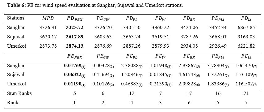
4.1 Power Density Error
Another selection criteria used for wind speed analysis was power density error (PE). This criterion was based on the relative difference of two average powers. One was mean power density (MPD) calculated from observations and other was mean power density (PDM) calculated from the model under study. The criterion was defined as
$$PE=\left|\frac{MPD-P{D}_{d}}{MPD}\right| \left(8\right)$$
The formula for \(MPD\) and \({PD}_{d}\) are defined respectively
$$MPD=\frac{1}{2m}\rho A\sum _{k=1}^{m}{z}_{i}^{3} \left(9\right)$$

Here, \(\rho =P/RT\) is air density (kg/m3) at sea level. The air density is proportional to surface pressure (P) and air temperature (T) while R is the proportionality gas constant with value\(287 (J/Kg)\). However, A represents turbine blade sweep area (m3), and d stands for the distribution of interest for example, PBX distribution.
A comparison was also made between coastal stations by using the power density error and results are listed in Table 6. Overall, it was found that the PBX and GW distribution had the least power density error as compared to the other competitor models for all the stations with less estimation cost and greater efficiency.
The choice of suitable probabilistic model with low estimation cost can be utilized significantly for the identification of wind speed characteristics and wind energy potentials. The PBX distribution was introduced as an alternate wind speed model of Weibull and other well-known distributions. We analyze the data taken from three coastal regions of Sindh (Sanghar, Sujawal and Umerkot), Pakistan at 60m height. We have made comparison of PBX distribution with GW, PL, W, BX, PLi and Li distribution and conclude that the PBX is more appropriate and best fitted model as compared to considered competitor models. The results based on the ranking of numerous good of fit measures indicate that the PBX distribution has flexible behavior and it can significantly be used as an alternative model as compared to other wind speed distribution. Furthermore, PBX distribution has least power density error for all wind farms; therefore, it can be utilized for future predictions and estimation of wind speed potential at wind farms.
Author Contributions
Usman R. M. has written the main text of the manuscript. Ilyas M. has provided graphs and analysis of the data sets. Both authors equally contribute to review the paper.
Funding
The research receives no external/internal funding
Data Availability
Link of the data sets have attached in the manuscript
Code Availability
Available after request
Ethics Approval
Not applicable.
Consent to Participate
Not applicable.
Consent for Publication
Not applicable.
Conflict of Interest
The authors declare that they have no conflict of interest.
- Ahmad, K., Fakhry, M., & Jaheen, Z. (1997). Empirical Bayes estimation of P (Y< X) and characterizations of Burr-type X model. Journal of statistical planning and inference, 64(2), 297-308.
- Ahmed, M. A., Ahmed, F., & Akhtar, W. (2010). Wind characteristics and wind power potential for southern coasts of Sindh, Pakistan. Journal of Basic and Applied Sciences, 6(2), 163Á168.
- Akaike, H. (1998). Information theory and an extension of the maximum likelihood principle Selected papers of hirotugu akaike (pp. 199-213): Springer.
- Akdağ, S. A., & Güler, Ö. (2015). A novel energy pattern factor method for wind speed distribution parameter estimation. Energy Conversion and Management, 106, 1124-1133.
- Akgül, F. G., Şenoğlu, B., & Arslan, T. (2016). An alternative distribution to Weibull for modeling the wind speed data: Inverse Weibull distribution. Energy Conversion and Management, 114, 234-240.
- Akpinar, S., & Akpinar, E. K. (2009). Estimation of wind energy potential using finite mixture distribution models. Energy Conversion and Management, 50(4), 877-884.
- Alam, M. M., Rehman, S., Meyer, J. P., & Al-Hadhrami, L. M. (2011). Review of 600–2500 kW sized wind turbines and optimization of hub height for maximum wind energy yield realization. Renewable and Sustainable Energy Reviews, 15(8), 3839-3849.
- Alavi, O., Sedaghat, A., & Mostafaeipour, A. (2016). Sensitivity analysis of different wind speed distribution models with actual and truncated wind data: A case study for Kerman, Iran. Energy Conversion and Management, 120, 51-61.
- Arslan, T., Acitas, S., & Senoglu, B. (2017). Generalized Lindley and Power Lindley distributions for modeling the wind speed data. Energy Conversion and Management, 152, 300-311.
- Bilir, L., İmir, M., Devrim, Y., & Albostan, A. (2015). An investigation on wind energy potential and small scale wind turbine performance at İncek region–Ankara, Turkey. Energy Conversion and Management, 103, 910-923.
- Burr, I. W. (1942). Cumulative frequency functions. The Annals of mathematical statistics, 13(2), 215-232.
- Chiodo, E., De Falco, P., Di Noia, L. P., & Mottola, F. (2018). Inverse Log-logistic distribution for Extreme Wind Speed modeling: Genesis, identification and Bayes estimation. AIMS Energy, 6(6), 926-948.
- Dupré, A., Drobinski, P., Alonzo, B., Badosa, J., Briard, C., & Plougonven, R. (2020). Sub-hourly forecasting of wind speed and wind energy. Renewable Energy, 145, 2373-2379.
- Johnson, N. L., Kotz, S., & Balakrishnan, N. (1995). Continuous univariate distributions, volume 2 (Vol. 289): John wiley & sons.
- Kantar, Y. M., Usta, I., Arik, I., & Yenilmez, I. (2018). Wind speed analysis using the extended generalized Lindley distribution. Renewable Energy, 118, 1024-1030.
- Kitaneh, R., Alsamamra, H., & Aljunaidi, A. (2012). Modeling of wind energy in some areas of Palestine. Energy Conversion and Management, 62, 64-69.
- Kolmogorov, A. (1933). Sulla determinazione empirica di una lgge di distribuzione. Inst. Ital. Attuari, Giorn., 4, 83-91.
- Mert, I., & Karakuş, C. (2015). A statistical analysis of wind speed data using Burr, generalized gamma, and Weibull distributions in Antakya, Turkey. Turkish Journal of Electrical Engineering & Computer Sciences, 23(6), 1571-1586.
- Morgan, E. C., Lackner, M., Vogel, R. M., & Baise, L. G. (2011). Probability distributions for offshore wind speeds. Energy Conversion and Management, 52(1), 15-26.
- Raqab, M. Z., & Kundu, D. (2006). Burr type X distribution: revisited. Journal of probability and statistical sciences, 4(2), 179-193.
- Rocha, P. A. C., de Sousa, R. C., de Andrade, C. F., & da Silva, M. E. V. (2012). Comparison of seven numerical methods for determining Weibull parameters for wind energy generation in the northeast region of Brazil. Applied Energy, 89(1), 395-400.
- Sarkar, A., Singh, S., & Mitra, D. (2011). Wind climate modeling using Weibull and extreme value distribution. International Journal of Engineering, Science and Technology, 3(5), 100-106.
- Smirnov, N. V. (1939). Estimate of deviation between empirical distribution functions in two independent samples. Bulletin Moscow University, 2(2), 3-16.
- Snedecor, G. W., & Cochran, W. G. (1967). Statistical Methods. Ames, Iowa: Iowa State University Press.
- Solaun, K., & Cerdá, E. (2020). Impacts of climate change on wind energy power–Four wind farms in Spain. Renewable Energy, 145, 1306-1316.
- Soukissian, T. (2013). Use of multi-parameter distributions for offshore wind speed modeling: The Johnson SB distribution. Applied Energy, 111, 982-1000.
- Surles, J., & Padgett, W. (2001). Inference for reliability and stress-strength for a scaled Burr Type X distribution. Lifetime data analysis, 7(2), 187-200.
- Surles, J., & Padgett, W. (2005). Some properties of a scaled Burr type X distribution. Journal of statistical planning and inference, 128(1), 271-280.
- Usman, R. M., & Ilyas, M. (2020). The Power Burr Type X Distribution: Properties, Regression Modeling and Applications. Punjab University Journal of Mathematics, 52(8), 27-44.
- Usta, I., & Kantar, Y. M. (2012). Analysis of some flexible families of distributions for estimation of wind speed distributions. Applied Energy, 89(1), 355-367.
Table 6 is available in the Supplementary Files section.
No competing interests reported.