4.1. Shear-wave velocity structure at the prediction site
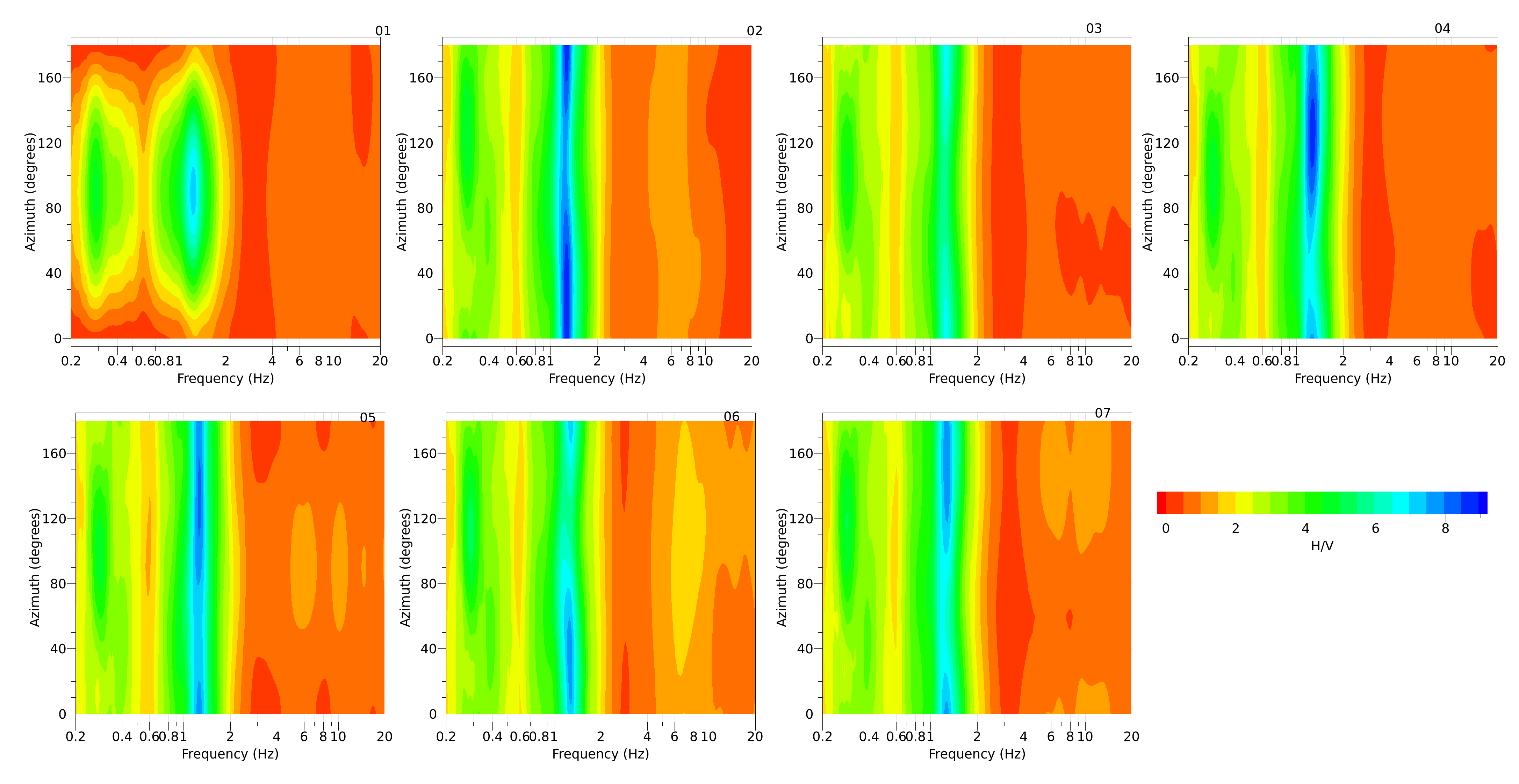
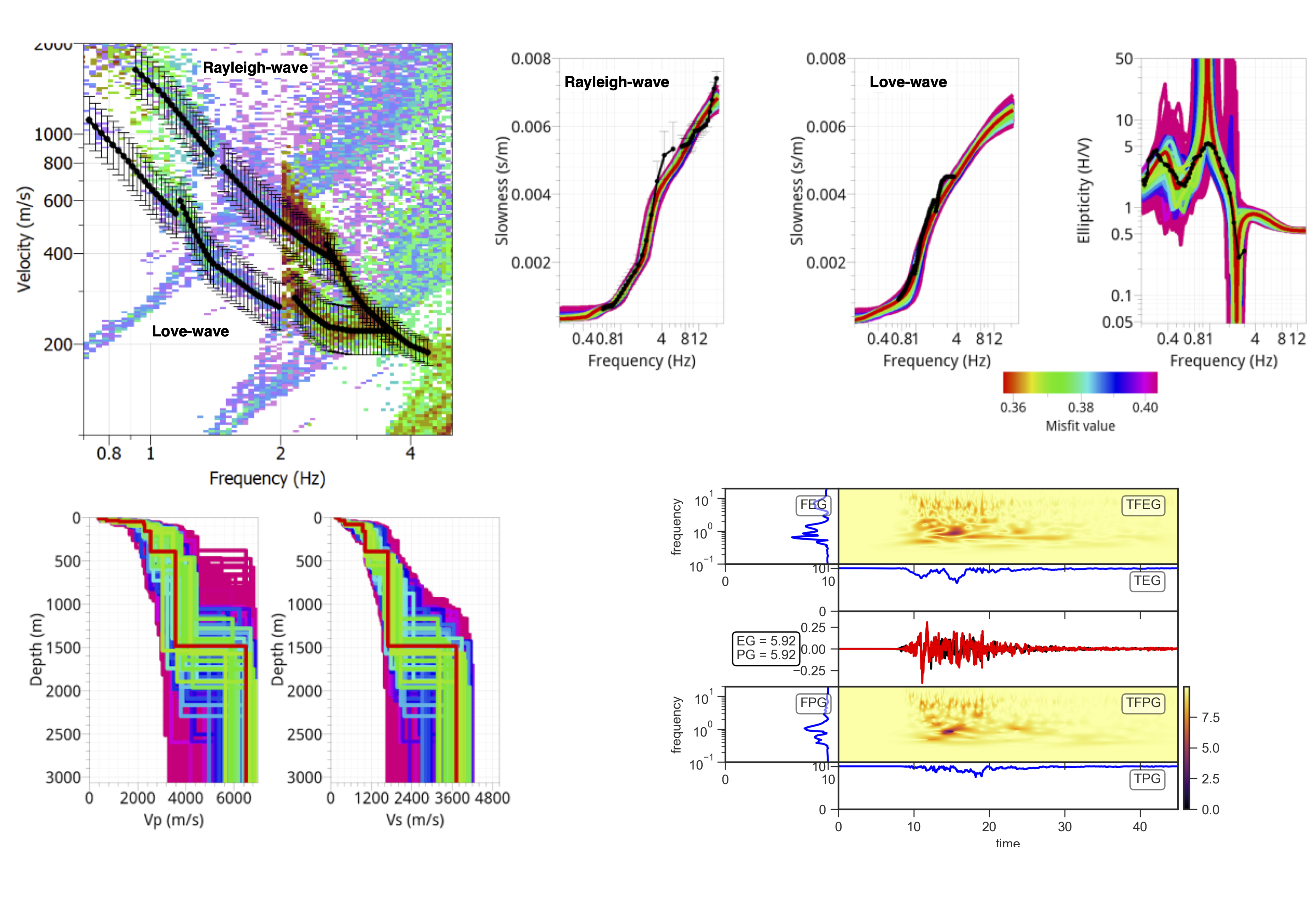
AMV data collected at the KUMA prediction site are characterized by a significant contribution of surface waves, and the use of arrays with increasing aperture allowed to derive surface-waves dispersion curve data in a wide frequency range (from 0.7 to 20 Hz). Moreover the geometry composed of two nested triangles using seven seismic stations proved very convenient since it allowed for good azimuthal coverage of surface-wave propagation fronts with a limited number of stations. We have adopted different techniques of analysis obtaining very consistent results in terms of fundamental mode Rayleigh-wave dispersion data (Fig. 9d). Further, the Raydec and RTBF analyses allowed to extract Rayleigh-wave ellipticity and the fundamental mode Love-wave dispersion curves, respectively.
The best fit model derived from the joint inversion of DC and ellipticity data shows a good agreement between experimental and theoretical curves, except in the frequency band 4–6 Hz where the theoretical Rayleigh DC is not able to follow the inflection of the experimental DC (Fig. 10). The ESG6 Committee has provided its “consensus” model for the target site based on literature data. We compared this “consensus” model with our results in Fig. 12, finding a satisfactory agreement between the two models. The first 400 m of the Vp and Vs profiles are very similar, and also the deep seismic contrast around a depth of 1500 m is found in both models. The main difference between the two is in the depth of the intermediate seismic velocity contrast, which is found at a depth of about 400 m in our model versus 600 m in the “consensus” model. On average, our model shows lower Vs values than the “consensus” one between 400 and 1500 m, and some discrepancies are also observed in the density values (which were fixed during our inversion). The comparison between the two models is also performed in terms of SH transfer functions (Fig. 12) computed by the reflectivity method (Kenneth and Kerry, 1979). Both functions point out that the main ground motion amplification should be observed in the 1–2 Hz frequency range, with SH transfer functions showing some differences in the amplification level, mainly in the lower frequency range (i.e. < 1 Hz) and between 1.5 and 2 Hz.
4.2. 1D simulation results
The 1D simulations predicted significant horizontal ground motion amplification at the KUMA site for both weak- and strong-motion input. For the M 5.9 earthquake (step2), the predicted time series by the EQL approach shows PGA of about 0.036 g for the EW component and of about 0.049 g for the NS component (Table 6 and Fig. 13c, d). Such prediction is in very good agreement with the observation for the EW ground-motion recorded at the KUMA site (0.034 g; Fig. 13a,c), whereas peak ground motion for the NS component is largely overestimated by 45% (Fig. 13b,d).
Table 6
Values of Peak Ground Acceleration (PGA) from observations at KUMA (obs), Strata EQL model (strata) and fully nonlinear model (deepsoil)
| | PGA EW component (g) | PGA NS component (g) |
| Mj 5.9 | 0.034 (obs) 0.036 (strata) | 0.031 (obs) 0.049 (strata) |
| Mj 6.5 | 0.396 (obs) 0.315 (strata) 0.183 (deepsoil) | 0.45 (obs) 0.317 (strata) 0.145 (deepsoil) |
The comparison of Fourier Amplitude Spectra (FAS) shows that the 1D EQL predictions have larger amplitude than the observations for frequencies below 3 Hz (Fig. 13g,h). This is particularly evident from the examination of the FAS calculated for the NS component of the ground motion in the frequency band 1–2 Hz (Fig. 13h). It is worth noting that in this frequency band, the NS input ground motion component has FAS amplitude 3 times larger than the EW input component, so large that the NS input FAS is comparable to that observed at KUMA (Fig. 13h), thus explaining the differential response predicted at the surface due to the two input motions.
This frequency dependent ground motion overestimation of the recordings by the 1D EQL predictions is pointed out by the comparison between observed and predicted 5% damped elastic response spectra (Fig. 13i,l). At KUMA, peaks of the recorded acceleration spectral ordinates (Sa) are observed in the period band between 0.1 and 0.4 s; the larger amplitudes were recorded for the NS ground motion component, with values around 0.13 g (Fig. 13l). In terms of Sa, the predictions largely overestimate the observed response spectra in the period-band 0.4–0.8 s, where the 1D EQL simulations show amplitudes up to 2.3 times larger than the observations for the EW ground-motion component (about 0.07 g, Fig. 13i) and up to 5 times larger for the NS ground-motion component (about 0.125 g, Fig. 13l).
To obtain a more quantitative evaluation of the goodness-of-fit (GoF) between predicted and recorded motions, we used the categories proposed by Kristekova et al. (2009), which are based on time-frequency (TF) representation of the waveforms to be compared and related misfit metrics. In particular, two indices are used to quantify the amplitude difference between signals based on their envelope quantitative comparison (EG), and the phase GoF (PG). To such aim, the predicted and recorded ground-motions were bandpass filtered between 0.1 and 20 Hz using a fourth-order non-causal butterworth filter before computation of their continuous wavelet transform (Daubechies, 1992), and the calculation of GoF metrics was through the obspy python package (Beyreuther et al. 2010). According to the original formulation of Kristekova et al. (2009), EG and PG, along with other GoF parameters, are allowed to vary in the range 0–10, where 10 means perfect agreement between observed and predicted ground-motion, values below 4 indicate a poor fit, values in the range 4–6 stand for a fair fit, values between 6 and 8 represent a good fit and over 8 are for an excellent fit.
For the Mj 5.9 predictions, the EG values are about 3.5 and 2.5 for the EW and NS horizontal components (Fig. 14), indicating a rather poor amplitude GoF with the observations, whereas the phase GoF is fair for the EW component (PG of about 4.8) and the NS component (PG of about 4). EG as a function of frequency (FEG, insets in Fig. 14) shows that the large amplitude misfit is between 1–2 Hz while PG as a function of frequency (FPG, insets in Fig. 14) shows that the phase-misfit is concentrated in a wide frequency band, especially for the NS component.
For the Mj 6.5 Kumamoto foreshock, we compared horizontal strong ground motion predictions obtained using the EQL and NL approaches with the observations. The observed peak acceleration value is about 0.40 and 0.45 g for the EW and NS components (Table 6 and Fig. 15a,b). The input ground motions recorded at SEVO show similar waveforms and PGA values, about 0.12 g for the EW component and 0.10 for the NS (Fig. 15g,h). The output PGA for the EQL simulations is about 0.32 g for both horizontal components (Fig. 15c,d), whereas the PGA is about 0.18 g for the EW component and 0.15 g for the NS component in the case of the NL predictions (Table 6 and Fig. 15e,f). The visual inspection of acceleration time series reveals a fairly good strong seismic phases alignment between predictions and observations; however, the same inspection highlights the strong low-pass filtering effect of 1D site modeling, particularly for the EQL ground-motion predictions (Fig. 15c,d). In fact, the comparison between FAS obtained by EQL and NL predictions and FAS observations at KUMA show that both 1D modeling approaches underpredict the recorded motions (Fig. 15i,l). The underprediction is larger for the NS than the EW component and for frequencies higher than about 5 Hz.
In terms of Sa, the recorded EW 5%-damped elastic response spectra show three main maxima: around 0.15 s, with amplitude of about 0.9 g, around 0.4 s, with amplitude of about 0.7 g and a broad peak centered around 1.0 s, with amplitude of about 0.75 g (Fig. 15m). For this component, the EQL prediction shows a fairly good agreement for the periods higher than 0.8 s. In fact, the 1D EQL simulated response spectra shows a similar broad peak centered around 1 s with amplitude which is only slightly underestimated (of about 7%) with respect to the observed. The main disagreement of Sa value is in the lower periods (T < 0.8 s), for which the observed Sa is up to 125% larger than the prediction (Fig. 15m). The NL simulation for the EW ground motion component severely underpredicts the observed response spectra in the period range 0.1–2.5 s, with amplitudes lower than 110% at 1.0 s and 125% at 0.15 s (Fig. 15m). Similar considerations hold for the predicted NS elastic response spectra; the shape of predicted and observed response spectra are similar but both EQL and NL predictions systematically underpredict the observed Sa in all periods bands, with larger discrepancies for the NL prediction (Sa amplitudes 2.5 times lower than observations at 0.8 s) (Fig. 15n). As a general consideration, the EQL predictions in terms of maximum Sa are 75% larger than the NL ones and thus show lower disagreement with the observed data (Fig. 15m,n).
We have calculated envelope (EG) and phase (PG) GoF between predicted and recorded horizontal motions also for the Mj 6.5 earthquake (Fig. 16) through the time-frequency misfit analysis of Kristekova et al. (2009). For this earthquake, we obtained larger GOF parameters with respect to the Mj 5.9 event. Amplitude GoF between predictions and recorded ground motion is fair (Fig. 16), with higher EG values (EG of about 5.9 for the EW and 5.7 for the NS components) for the 1D EQL motions with respect to the 1D NL (EG lower than 5.5). Phase GoF is good for both EQL and NL models; the higher values of PG are obtained for the NS component predictions (PG of about 6.8 and 6.7 for the EQL and NL simulations) with respect to the EW (PG of about 6.0 and 6.4 for the EQL and NL simulations).
For the Kumamoto foreshock, we also calculated the maximum shear strain vertical profile obtained by EQL and NL simulations; for both approaches, the peak strain is reached at the same depth around 37 m, where the implemented Vs model jumps from about 250 m/s to 400 m/s (corresponding to the bottom part of layer #7 in Tables 4 and 5). The differences in terms of strain profile between the two approaches are shown in Fig. 17; for the EW component, the peak shear-strain calculated with the EQL approach (about 0.2%) is about double that of the NL one (Fig. 17 left panel). For the NS component the differences are lower, the peak strain is about 0.16% for the NL case whereas it is 0.22% for the EQL case.
In terms of site transfer function, it is remarkable to note that there is a substantial agreement between the estimates of the main site amplification frequency, around 1.2 Hz, obtained by empirical methods, namely the SSR and EHV, applied to weak ground motions (Mj < 5) and the theoretical site transfer function (TTF), which is calculated as spectral ratio between FAS input ground motion and FAS surface EQL prediction at KUMA (Fig. 18). In particular, the denominator of the TTF is also calculated using weak input motions recorded at SEVO for earthquakes with Mj < 5 (Table 1); for such input motions the calculated TTFs overlap and the soil nonlinear behavior is negligible (the maximum shear strain is equal to 0.015% in our EQL prediction and is reached for the NS component at a depth of about 37 m). The agreement between all three curves is satisfactory in the range 1–2 Hz. Beyond this frequency, the EHV shows lower amplitudes with respect to the SSR, which is considered a more robust estimator of the site amplification function. The agreement between TTF and the average SSR extends to higher frequency up to 4 Hz, where the TTF remains within the uncertainty range of the SSR curve. At higher frequencies, the SSR shows substantially higher amplitudes (up to 2.5 times larger at 7.5 Hz) than both EHV and TTF up to 9 Hz (Fig. 18). Above 10 Hz, the average empirical transfer functions and TTF fall within the average ± 1𝝈 bounds of the expected value and reduce with increasing frequency. It is worth noting that the empirical amplification functions did not pointed out any clear low frequency peak around 0.3 Hz as shown in the H/V curve based on AMV data, likely because of the different sensitivity of the instrumentation used to record earthquake signals at the KUMA site (accelerometer) and AMV (short period sensors) and likely due to the short time-windows used to analyze the earthquake data.