Epilepsy is a neurological disorder that causes seizures and involves widespread structural alteration. Magnetic resonance (MR) is the preferred imaging tool for investigating patients with epilepsy and is also used for segmentation. We used to compare QuickNAT and FSL-FIRST software for the segmentation of subcortical structures in patients with temporal lobe epilepsy (TLE-R and TLE-L) and healthy control. We found that there were statistically significant differences among the automated methods in all groups (TLE-R, TLE-L, and control; mean ± SD) at the left pallidum (16.397 ± 9.326; 18.333 ± 11.062;39.322 ± 23.711) left putamen (29.561 ± 13.642;27.713 ± 13.696;22.499 ± 7.994), right amygdala (26.173 ± 19.743;22.822 ± 12.787;19.429 ± 11.617), right pallidum (24.205 ± 11.674;24.706 ± 10.647;38.976 ± 20.405), and right putamen (37.223 ± 19.498;31.143 ± 18.714;20.914 ± 9.885). We found the superiority of FSL-FIRST software over QuickNAT in calculating both volumes (raw and normalized) of subcortical structures.
Article
Comparison of QuickNAT and FSL-FIRST for segmentation of subcortical structures in patients with epilepsy
https://doi.org/10.21203/rs.3.rs-2213842/v1
This work is licensed under a CC BY 4.0 License
Version 1
posted
You are reading this latest preprint version
Epilepsy is a neurological disorder that causes seizures and involves widespread structural alteration. Clinical presentation varies between epileptic syndromes, affecting about 0.6–1.5% of the population worldwide [1]. About one-third of all patients with epilepsy poorly respond to antiepileptic drug therapy, i.e., seizures are not controlled by two or more appropriately chosen antiepileptic medications or other therapies [2]. A seizure is an event that occurs when there is a distortion of the normal balance between cortical excitation and inhibition in the brain. Since the mid-20th century, researchers have hypothesized the role of subcortical structures in seizure generation. Penfield and Jasper postulated that the thalamus and upper brain stem are critical in ictogenesis [3]. Current data suggest that subcortical structures play an important role in the propagation and behavioral manifestation of an epileptic seizure [4].
Currently, magnetic resonance (MR) is the preferred imaging tool for investigating patients with epilepsy. With the development of new diagnostic approaches based on artificial intelligence, data from MR imaging have been recognized as important input data for machine learning. The advantages of machine learning over conventional methods include precise and automated learning, which can be used to create practical algorithms for clinical medicine and basic research [5–7]. Many algorithms have been developed for the segmentation of subcortical structures. These algorithms are automated, freely available, and have been employed in several extensive MR imaging studies [8, 9]. T1-weighted MR images of the human brain are used for segmentation. These images have three-dimensional isotropic voxels and full head coverage. Every voxel has an intensity value typically represented on a grayscale from 0 to 255. Volumes of postprocessing subcortical structures are calculated as the sum of the image intensity at the voxels belonging to a specific tissue structure and the proportion of voxel volume occupied by each tissue. Manual segmentation by experts is a gold standard, but it is subject to inter- and intraobserver bias [10–12]. Moreover, manual segmentation requires significant time for the volumetric quantification of a large dataset. In contrast, automatic segmentation reduces processing time and facilitates the analysis of a large amount of data. Factors that can affect the reproducibility of segmentation methods are imaging protocols, different models of MR machines, subjects’ positions during imaging, image artifacts because of moving patients, and partial volume averaging [13–16].
In this study, we compared the reproducibility of automatic brain segmentation algorithms that employ different template strategies, including QuickNAT (a fully convolutional neural network, F-CNN) and FIRST (which uses a model-based single atlas). We hypothesized that the two different segmentation algorithms would exhibit differing levels of reproducibility and that FSL-FIRST overcomes QuickNAT.
Participants
The neurologist made a diagnosis of temporal lobe epilepsy (TLE) through clinical exams and EEG monitoring. All patients have an MRI exam. Structural MR images (n = 118) were obtained from individuals aged 13–59 years at the Clinic of Neurology, University Clinical Center of Serbia, Belgrade. The participants included 54 men (45.8%) and 64 women (54.2%). They encompassed individuals with temporal lobe epilepsy (TLE) (n = 80) and healthy participants (n = 38). Individuals with TLE were divided into two groups, the TLE-R group (n = 28) and the TLE-L group (n = 52). The TLE-R group included 14 men (50%; mean age, 31.3 ± 7.6 years) and 14 women (50%; mean age, 30.4 ± 7.9 years). The TLE-L group included 29 men (55.8%; mean age, 35.6 ± 9.1 years) and 23 women (44.2%; mean age, 34.3 ± 10.2 years). Healthy participants included 17 men (44.7%; mean age, 27.3 ± 6.2 years) and 21 women (55.3%; mean age 35.7 ± 9.9 years.
Mr Imaging Data
The T1-weighted (T1w) MR imaging sequence was used for anatomical characterization. High-resolution structural scans were acquired in the sagittal plane at 1.5 T (Philips Achieva, Amsterdam, Netherlands), 1.5 T (Siemens, Avanto/Aera, Erlangen, Germany), and 3 T (Siemens Skyra, Erlangen, Germany). The imaging parameters were as follows: TR = 25ms, flip angle = 8°, acquisition matrix of 256×232×180 (for 1.5 T Philips); TR = 1700ms, flip angle = 4°, acquisition matrix of 240×256×180 (for 1.5 T Siemens); and TR = 1700ms, flip angle = 5°, acquisition matrix of 240×256×180 (for 3 T Siemens). The voxel size for all three MRI machines was 1×1×1 mm3.
Segmentation Methods
QuickNAT segmentation
Quick segmentation (QuickNAT) software is based on a deep fully convolutional neural network (F-CNN). Its postprocessing times run in seconds and use three two-dimensional F-CNNs, where each operates in a separate plane (transversal, sagittal, and coronal). The first step of making QuickNAT was to apply the existing software FreeSurfer [17] to segment scans without annotations. After that, the software was used to continue training the previous network with smaller manually annotated data to achieve high segmentation accuracy. QuickNAT was the first to utilize the publicly available software (FreeSurfer) to segment the data and train the network. The authors reported high test-retest accuracy, which makes it suitable for longitudinal studies. The final segmentation and labels correspond to 27 brain structures (cortical and subcortical). The code and trained model are available as extensions of MatConvNet [18] at https://github.com/abhi4ssj/QuickNatv2.
Fsl-first Segmentation
A commonly used, automated, model-based approach is the FMRIB Integrated Registration and Segmentation Tool (FIRST), which is provided as a part of the FSL software library [15].
The construction of the model was based on a manually labeled dataset [19]. It first registers the images to MNI152 space by performing affine registration. FSL-FIRST [20] is one of the most commonly used algorithms for the segmentation of subcortical structures and has been validated by the scientific community [21, 22]. It uses a model-based single atlas that runs approximately about 15 minutes. Before starting segmentation, we used the “fslreorient2std” script to ensure the adequate orientation of the images. The “run_ first_all” script was applied to automatically segment subcortical structures into 15 different labels. The fully automated segmentation of the volumes is available at http://fsl.fmrib.ox.ac.uk/. We used FSL-FIRST v.6.0.3.
Quality Control Of Segmentation
Segmentations with gross errors were excluded from further investigation. These errors typically happened due to a major failure of the atlas to target image registration. Images requiring exclusion were images where the segmentation region of interest (ROI) did not overlap with anatomical brain boundaries. All segmentation images have a visual inspection.
Determination Of Common Roi Labels
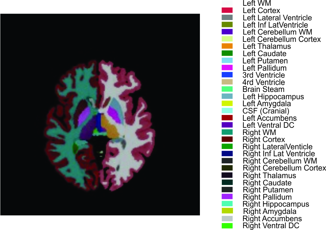
A direct comparison of an ROI is not possible because the references of labels and the delineation of boundaries of anatomical regions are different between QuickNAT [17] and FSL (Harvard-Oxford atlas). Therefore, we used a FreeSurfer space for overlapping the results of the segmentation of these two different methods. The set of ROIs included the following subcortical structures: thalamus (L + R), caudate (L + R), putamen (L + R), pallidum (L + R), and amygdala (L + R). Matched ROIs were inspected by one manual rater (Z.J.) based on the ROI’s names and spatial correspondence between them. A visualization of the ROIs and list of matched ROIs at QuickNAT and FSL-FIRST is presented in Fig. 1 and Fig. 1A.
Statistical analysis
Statistical analyses were performed in Rstudio software (version 1.4.1106). The percentage volume difference (PVD) was calculated by using the following formula:
$$PVD=100 x \frac{|V\left(A\right)-V\left(B\right)|}{\frac{V\left(A\right)+V\left(B\right)}{2}}$$
where V(A) and V(B) were volumes obtained by using FSL and QuickNAT, respectively.
Comparison between volumes obtained by different techniques (parameters – brain segmentations) on the same group of subjects (separately TLE-R, TLE-L, and control) was done by using paired t test or Wilcoxon test. t test was used when the normality of the distribution is satisfied, and Wilcoxon test when is not. Kruskall-Wallis test was used to determine whether or not a statistically significant difference exists between TLE-R, TLE-L, and the control group of subjects. For pairwise comparisons between each independent group, if the results of Kruskall-Wallis test were statistically significant, was used Dunn’s test. The Bonferroni correction was used for Dunn’s test, so the p-values considered significant only if it was smaller than 0.05/3 = 0.017.
Bonferroni correction was used because we had multiple comparations. In our study, we had a 10 comparison and needed to divide with a limit value (p < 0.05). That is a reason why p < 0.005 was considered significant. Intraclass correlation coefficients (ICCs) were calculated to describe the consistency between the volumes obtained from FSL and QuickNAT. An ICC calculation two-way mixed model was selected. An ICC value of 1 indicated perfect reproducibility between the two methods, while a value of 0 suggested reproducibility lower than expected based on chance alone.
The Dice coefficients are a statistical test used for the validation of imaging segmentation algorithms. We used FSL-FIRST as a gold standard because it has been validated in the scientific field. The Dice coefficient represents the spatial overlap index. The value ranges from 0, which indicates no spatial overlap between the two segmentation methods, to 1, which indicates complete overlap. The Dice coefficients (D) were calculated by using the following formula:
$$D=2*\frac{|X\bigcap Y|}{\left|X\right|+\left|Y\right|}$$
where X and Y were segmentations obtained by using FSL and QuickNAT, respectively; |X| and |Y| means the number of elements in that set (X or Y); ⋂ represented the intersection of the two segmentation methods; and means of the elements that are common in both methods.
Dice coefficients. The Dice coefficients measure the similarity by overlapping two different segmentation methods. QuickNAT used the mgz format for the results of segmentation in the FreeSurfer environment, while FSL used the gz/vtk format. Therefore, we first had to convert the FSL-FIRST image to mgz format. After that, we calculated the Dice coefficients in FreeSurfer space using the command mri_seg_overlap for both methods in each group participant. The Dice coefficient was less than 0.01, indicating that there was no spatial overlap between these two methods.
PVD. PVD is used for the relative quantification of volume differences between two segmentation methods. The minimum value for PVD is zero. A higher PVD indicated a greater volume difference between the two segmentation methods. We calculated PVD from the raw volumes of every participant in both segmentation methods. The results are presented in Table 1. Specifically, in the TLE-R group, there were statistically significant differences among the automated methods in the left amygdala, left pallidum, left putamen, right amygdala, right pallidum, and right putamen. In the TLE-L group, significant inter-method differences were found in the left pallidum, left putamen, right amygdala, right pallidum, and right putamen. In the control group, there were inter-method differences in the left amygdala, left caudate, left pallidum, left putamen, right amygdala, right caudate, right pallidum, and right putamen.
Volumetric differences. For the volumetric differences among the segmentation methods, we used Bonferroni correction at p<0.005. The results are presented in Table 2. Significant volumetric differences between the two groups (TLE-R and TLE-L) and healthy controls were found. Specifically, with the FSL-FIRST method, there were lower volumes in both TLE groups across regions including left caudate, left putamen, left pallidum, right caudate, and right pallidum. The QuickNAT method showed lower volume in both TLE groups compared to the control group only in the left and right putamen.
ICC. ICCs indicate the consistency and absolute agreement between the QuickNAT and FSL-FIRST segmentation methods. The ICC values can range from 0 to 1, with 0 (no consistency among segmentation methods) and 1 (perfect consistency). Values lower than 0.5 indicate poor consistency, those between 0.5 and 0.75 indicate moderate consistency, those between 0.75 and 0.9 indicate good consistency, and those higher than 0.9 indicate excellent consistency [23].
In the TLE-R group, there was good consistency for the right thalamus (0.809) and left thalamus (0.799), and moderate consistency for the left caudate (0.709), left pallidum (0.519), right caudate (0.550), and right putamen (0.610). In the TLE-L group, there was moderate consistency for the left thalamus (0.648), left caudate (0.725), left putamen (0.534), left amygdala (0.522), and right caudate (0.646). In the control group, there was moderate consistency only for the left putamen (0.645) and right putamen (0.521). The results are presented in Table 3.
Segmentation of structural brain MRI analysis represents the classification of MRI data to specific tissue types and the identification of specific anatomical structures. QuickNAT belongs to the most used Bayesian classifier. The Bayesian classifier models the probabilistic relationship between the attribute set and the class variables, which are then used for estimating the class probability of the unknown variable [24]. While, FSL used atlas-based methods that are similar to classifier methods, except that they are implemented in the spatial domain rather than in the feature space. The atlas contains information about the brain anatomy and it is used as a reference for segmenting new images [25].
In this study, we examined the reliability of two noncommercial automatic programs (QuickNAT and FSL-FIRST) for the segmentation of subcortical structures in groups of patients with epilepsy and healthy subjects. FSL-FIRST is one of the most often used tools in neuroimaging segmentation, which is why we considered this method the gold standard. We also examined the differences in normalized and raw volumes between subcortical structures in patients with TLE and healthy controls.
Given that QuickNAT (F-CNN) ran segmentation within a few seconds, it was faster than FSL-FIRST (atlas-based), which needed about 15 minutes for the segmentation of subcortical structures. With the FSL-FIRST method, both TLE groups showed abnormalities in the ipsilateral pallidum compared with the control group, supporting the notion that TLE has a specific network that extends beyond the mesial temporal lobes [26]. With the QuickNAT, the difference was only significant at both putamens, and it did not show differences in the volume of the thalamus which are typical for TLE [27].
Calculating raw volume on subcortical structures we found an ipsilateral difference in the volume of the thalamus. This is important because the thalamus is a major hub in the epilepsy network [28,29]. Some authors suggested that a loss of forwarding inhibition between the thalamus and neocortical connections may be epileptogenic [30].
Subcortical structures shows generally higher volumes at 3T vs. 1.5T, especially for raw volumes. 3T showed slightly better sensitivity than 1.5T for atrophy of subcortical structures. For normalized volumes, 3T MR detected atrophy in the globus pallidus but 1.5T did not. Results of volumetric data can be obtained from postprocessing and can be included in prognostic models of treatment outcomes [31,32].
Our study has some limitations. We did not manually calculate volumes from our data to be considered a gold standard and compare them with these two segmentation methods. One more limitation is that we used different hardware and variable sequence parameters. Previous multicentre neuroimaging studies found that even similar imaging protocols can obtain the differences in structural segmentation data. This variability produces datasets characterized by different signal-to-noise ratios, which in turn might alter the automatic segmentation results [31].
The success of deep learning is mainly by supervised learning, while unsupervised approaches are still a field of research. Also, the atlas-based automatic segmentation method gave us more realistic results than the algorithm that used more network layers. Maybe the problem is that convolutional neural networks need more training data for better results.
In this study, we found the superiority of FSL-FIRST software over QuickNAT in calculating both volumes (raw and normalized) of subcortical structures. These results are opposed to already existing research papers about QuickNAT. Atlas-based methods are still superior to the classifier models.
Ethical approval
All procedures performed in the studies involving human participants were in accordance with the ethical standards of the institutional and/or national research committee and the 1964 Helsinki declaration and its later amendments or comparabe ethical standards. This retrospective study was approved by the Research Ethics Committee of the University Clinical Center of Serbia (application number 971/4/22/09/2022).
Consent to participate
Written informed consent was obtained from all participants and their guardians if necessary.
Consent for publications
All of the authors have approved the content of this paper and have agreed to the Scientific Reports’ submission policies as well as the responsible authorities as the institute where the research has been carried out.
Acknowledgments
The research was supported by the Ministry of Education, Science and Technological Development of the Republic of Serbia (contact 451-03-68/2022-14/200103).
We thank the Center for Magnetic Resonance Imaging at the University Clinical Centre Serbia for sharing data.
Author contributions
Z.J., A.P., and A.R. designed the study. D.S. and N.V. recruited the study patients and collected the clinical data. Z.J. and M.M. analyzed MRI imaging that is satisfactory for postprocessing. Z.J. was done all postprocessing. V.M.J. was done completely statistical analysis. All the authors interpreted the data. Z.J. drafted the first version of the manuscript, and all the authors participated in revising the manuscript. All the authors approved the final manuscript.
Data availability
The datasets generated and/or analyzed during the current study are available from the corresponding author upon reasonable request.
Competing interests
The authors declare no competing interests.
- Bell GS, Neligan A, Sander JW. An unknown quantity--the worldwide prevalence of epilepsy. Epilepsia. 2014 Jul;55(7):958-62. doi: 10.1111/epi.12605. Epub 2014 Jun 25. PMID: 24964732.
- French JA. Refractory epilepsy: a clinical overview. Epilepsia 2007; 48 Suppl 1:3–7. doi: 10.1111/j.1528-1167.2007.00992.x. PMID: 17316406.
- Penfield, W. and Jasper, H. (1954) Epilepsy and the Functional Anatomy of the Human Brain. Little, Brown, Boston, 363-365.
- Badawy RA, Vogrin SJ, Lai A, Cook MJ. The cortical excitability profile of temporal lobe epilepsy. Epilepsia. 2013 Nov;54(11):1942-9. doi: 10.1111/epi.12374. Epub 2013 Sep 20. PMID: 24112043.
- Middlebrooks E.H., Ver Hoef L., Szaflarski J.P. Neuroimaging in epilepsy. Curr. Neurol. Neurosci. Rep. 2017;Apr;17(4):32. doi: 10.1007/s11910-017-0746-x. PMID:28324301
- Jin B., et al. Automated detection of focal cortical dysplasia type II with surface-based magnetic resonance imaging postprocessing and machine learning. Epilepsia. 2018 May;59(5):982–992. doi: 10.1111/epi.14064. Epub 2018 Apr 10. PMID: 29637549; PMCID: PMC5934310..
- Wang W., et al. Voxel-based morphometric MRI postprocessing in non-lesional pediatric epilepsy patients using pediatric normal databases. Eur. J. Neurol. 2019 Jul;26(7):969-e71. doi: 10.1111/ene.13916. Epub 2019 Mar 12. PMID: 30685877.
- van Erp, T. G., et al. Subcortical brain volume abnormalities in 2028 individuals with schizophrenia and 2540 healthy controls via the ENIGMA consortium. Molecular Psychiatry. 2016 Apr;21(4), 547–553. doi.org/10.1038/mp.2015.63. Epub 2015 Jun 2. Erratum in: Mol Psychiatry. 2016 Apr;21(4):585. Pol, H E H [Corrected to Hulshoff Pol, H E]. PMID: 26033243; PMCID: PMC4668237.
- Hibar, D. P., et al. Subcortical volumetric abnormalities in bipolar disorder. Molecular Psychiatry. 2016; 21(12), 1710–1716. doi.org/10.1038/ mp.2015.227.
- Hoyte L., et al. Segmentations of MRI images of the female pelvic floor: a study of inter-and intra-reader reliability. J Magn Reson Imaging 2011 Mar;33(3):684-91. doi: 10.1002/jmri.22478. PMID: 21563253; PMCID: PMC4364418.
- Warfield S., et al. Automatic identification of grey matter structures from MRI to improve the segmentation of white matter lesions. J Image Guid Surg 1995;1(6):326-38. doi: 10.1002/(SICI)1522-712X(1995)1:6<326::AID-IGS4>3.0.CO;2-C. PMID: 9080353.
- Clark KA., et al. Impact of acquisition protocols and processing streams on tissue segmentation of T1 weighted MR images. Neuroimage 2006 Jan 1;29(1):185-202. doi: 10.1016/j.neuroimage.2005.07.035. Epub 2005 Aug 31. PMID: 16139526.
- Han X., et al. Reliability of MRI-derived measurements of human cerebral cortical thickness: the effects of field strength, scanner upgrade and manufacturer. Neuroimage. 2006 Aug 1;32(1):180-94. doi: 10.1016/j.neuroimage.2006.02.051. Epub 2006 May 2. PMID: 16651008.
- Gronenschild EH., et al. The effects of FreeSurfer version, workstation type, and Macintosh operating system version on anatomical volume and cortical thickness measurements. PLoS One 2012;7(6):e38234. doi: 10.1371/journal.pone.0038234. Epub 2012 Jun 1. PMID: 22675527; PMCID: PMC3365894.
- Patenaude B., et al. A Bayesian model of shape and appearance for subcortical brain segmentation. Neuroimage 2011;56:907-22. doi. org/10.1016/j.neuroimage.2011.02.046. Epub 2011 Feb 23. PMID: 21352927; PMCID: PMC3417233.
- Lehmann M., et al. Atrophy patterns in Alzheimer’s disease and semantic dementia: a comparison of FreeSurfer and manual volumetric measurements. Neuroimage 2010 Feb 1;49(3):2264-74. doi: 10.1016/j.neuroimage.2009.10.056. Epub 2009 Oct 27. PMID: 19874902.
- Fischl B., et al. Whole brain segmentation: automated labeling of neuroanatomical structures in the human brain. Neuron. 2002 Jan 31;33(3):341-55. doi: 10.1016/s0896-6273(02)00569-x. PMID: 11832223.
- Vedaldi, A. and Lenc, K. (2015) MatConvNet: Convolutional Neural Networks for MATLAB. Proceedings of the 23rd ACM International Conference on Multimedia, Brisbane, 26-30 October 2015, 689-692. doi.org/10.1145/2733373.2807412.
- Filipek, P. A., Richelme, C., Kennedy, D. N., & Caviness, V. S. Jr. (1994 The young adult human brain: an MRI-based morphometric analysis. Cerebral Cortex. 1994 Jul-Aug; 4(4), 344–360. doi: 10.1093/cercor/4.4.344. PMID: 7950308.
- Tae WS., et al. Validation of hippocampal volumes measured using a manual method and two automated methods (FreeSurfer and IBASPM) in chronic major depressive disorder. Neuroradiology 2008 Jul;50(7):569-81. doi: 10.1007/s00234-008-0383-9. Epub 2008 Apr 15. PMID: 18414838.
- Nugent AC, Luckenbaugh DA, Wood SE, et al. Automated subcortical segmentation using first: test–retest reliability, interscanner reliability, and comparison to manual segmentation. Hum Brain Mapp 2013 Sep;34(9):2313-29. doi: 10.1002/hbm.22068. Epub 2012 Jul 19. PMID: 22815187; PMCID: PMC3479333.
- Babalola KO., et al. Comparison and evaluation of segmentation techniques for subcortical structures in brain MRI. Med Image Comput Comput Assist Interv 2008;11(Pt 1): 409-16. doi: 10.1007/978-3-540-85988-8_49. PMID: 18979773.
- Koo TK, Li MY. A guideline of selecting and reporting intraclass correlation coefficient for reliability research. J Chiropr Med. 2016 Jun; 15(2):155-63. doi.org/10.1016/j.jcm.2016.02.012. Epub 2016 Mar 31. Erratum in: J Chiropr Med. 2017 Dec;16(4):346. PMID: 27330520; PMCID: PMC4913118.
- W. M. Wells III, W. E. L. Crimson, R. Kikinis, and F. A. Jolesz, “Adaptive segmentation of MRI data,” IEEE Transactions on Medical Imaging. 1996;15(4): 429–442. doi: 10.1109/42.511747. PMID: 18215925.
- Despotović I, Goossens B, Philips W, “MRI segmentation of the Human Brain: Challenges, Methods and Applications,” Computation and Mathematical Methods in Medicine 2015;2015:450341. doi 10.1155/2015/450341. Epub 2015 Mar 1. PMID: 25945121; PMCID: PMC4402572.
- de Campos BM, Coan AC, Lin Yasuda C, Casseb RF, Cendes F. Large-scale brain networks are distinctly affected in right and left mesial temporal lobe epilepsy. Hum Brain Mapp. 2016 Sep;37(9):3137-52. doi: 10.1002/hbm.23231. Epub 2016 May 2. PMID: 27133613; PMCID: PMC5074272.
- Whelan CD., et al. Structural brain abnormalities in the common epilepsies assessed in a worldwide ENIGMA study. Brain. 2018 Feb 1;141(2):391-408. doi: 10.1093/brain/awx341. PMID: 29365066; PMCID: PMC5837616.
- He X, Doucet GE, Pustina D, Sperling MR, Sharan AD, Tracy JI. Presurgical thalamic “hubness” predicts surgical outcome in temporal lobe epilepsy. Neurology 2017 Jun; 13;88(24): 2285–93. doi: 10.1212/WNL.0000000000004035. Epub 2017 May 17. PMID: 28515267.
- Jobst BC, Cascino GD. Thalamus as a "hub" to predict outcome after epilepsy surgery. Neurology. 2017 Jun 13;88(24):2246-2247. doi: 10.1212/WNL.0000000000004043. Epub 2017 May 17. PMID: 28515273.
- Paz JT, Huguenard JR. Microcircuits and their interactions in epilepsy: is the focus out of focus? Nat Neurosci. 2015 Mar;18(3):351-9. doi: 10.1038/nn.3950. PMID: 25710837; PMCID: PMC4561622.
- Chu R, Hurwitz S, Tauhid S, Bakshi R. Automated segmentation of cerebral deep gray matter from MRI scans: effects of field strength on sensitivity and reliability. BMC Neurology 2017 Sep 5;17(1):172. doi 10.1186/s12883-017-949-4. PMID: 28874119; PMCID: PMC5584325.
- Buchanan C., et al. Comparison of structural MRI brain measures between 1.5 and 3T: Data from the Lothian Birth Cohort 1936. Hum Brain Mapp. 2021 Aug; 15;42(12):3905-3921. doi:10.1002/hbm.25473. Epub 2021 May 19. PMID: 34008899; PMCID: PMC8288101.
Table 1.
Percentage volume difference (PVD) between the segmentation methods. Whiskers are set at minimum and maximum, and the horizontal line marks the median, whereas the box indicates the interquartile range (25-75%).

Table 2.
Comparison of volumetric difference as derivated from both segmentation techniques (Bonferroni correction at p<0.005).

Table 3.
ICC’s indicate the consistency and agreement between the QuickNAT and FSL-FIRST segmentation methods. Values >0.5 indicate poor consistency, those between 0.5 - 0.75 indicate moderate, those between 0.75 - 0.9 indicate good, and those < 0.9 indicate excellently.
|
ICC |
|||
|
ROI |
TLE-R |
TLE-L |
Control |
|
Left thalamus |
0,799 |
0,648 |
0,186 |
|
Left caudate |
0,709 |
0,725 |
0,343 |
|
Left putamen |
0,453 |
0,534 |
0,645 |
|
Left pallidum |
0,519 |
0,419 |
0,099 |
|
Left amygdala |
0,251 |
0,522 |
0,251 |
|
Right thalamus |
0,809 |
0,441 |
0,172 |
|
Right caudate |
0,55 |
0,646 |
0,237 |
|
Right putamen |
0,61 |
0,319 |
0,521 |
|
Right pallidum |
0,308 |
0,421 |
0,058 |
|
Right amygdala |
0,131 |
0,189 |
0,417 |
No competing interests reported.
- Figure1A.jpg
Figure 1A. ROI atlas denoting postprocessing structures in QuickNAT.