3.1. Design-Expert and analysis of results
There are two factors for making a super-waterproof coating: rough surface and rough surface correction. The StÖber method is one of the methods for synthesizing silica nanoparticles to make a rough surface. The purpose of designing the experiment is to optimize the parameters of the StÖber method to create a suitable rough surface and a surface modifying agent for the superhydrophobic coating. Finally, TEOS was investigated as a fixed precursor and the effect of deionized water (A), ethanol (B), ammonia (C), and PDMS (D). The central composite design (CCD) method was used for the design.
In this method, the experimental design is performed by specifying the actual levels and coding levels for each parameter (ie for high levels + 1, central levels zero, and low levels − 1). Actual and coded levels are shown in Table 1. The experimental design matrix with the levels encoded by the software is shown in Table 2. The obtained contact angle was entered into the software as a response.
Table 1
Actual levels and coded reaction parameters
| Factors | Code and Level |
| -1 | 00 | + 1 |
| A: Distilled water | 8 | 10 | 12 |
| B: Ethanol | 10 | 12 | 14 |
| C: Ammonia | 6 | 9 | 12 |
| D: Polydimethylsiloxane | 20 | 30 | 40 |
Table 2
Experimental design matrix with coded surfaces
| RUN | Factors | WCA Actual |
| | A | B | C | D | |
| 1 | 0 | -2 | 0 | 0 | 125.7 |
| 2 | -1 | 1 | -1 | -1 | 119.2 |
| 3 | -1 | 1 | 1 | -1 | 132.9 |
| 4 | -1 | -1 | 1 | 1 | 142.4 |
| 5 | 2 | 0 | 0 | 0 | 130.7 |
| 6 | 0 | 0 | 0 | 0 | 166.5 |
| 7 | 0 | 0 | 0 | 0 | 165.5 |
| 8 | -1 | 1 | -1 | 1 | 112.7 |
| 9 | -1 | -1 | -1 | -1 | 117.3 |
| 10 | -1 | 1 | 1 | 1 | 110.4 |
| 11 | -2 | 0 | 0 | 0 | 118.5 |
| 12 | 0 | 0 | 0 | 0 | 164.5 |
| 13 | 0 | 0 | 0 | 0 | 165.8 |
| 14 | 0 | 2 | 0 | 0 | 121.5 |
| 15 | 1 | 1 | 1 | 1 | 125.8 |
| 16 | 0 | 0 | 0 | -2 | 137.9 |
| 17 | -1 | -1 | 1 | -1 | 136.2 |
| 18 | 1 | 1 | -1 | 1 | 139.7 |
| 19 | 1 | 1 | 1 | -1 | 146.1 |
| 20 | 1 | -1 | -1 | 1 | 145.1 |
| 21 | 0 | 0 | 0 | 0 | 166.3 |
| 22 | 0 | 0 | 2 | 0 | 132.8 |
| 23 | 1 | -1 | -1 | -1 | 112.4 |
| 24 | 0 | 0 | 0 | 2 | 142.4 |
| 25 | 0 | 0 | 0 | 0 | 165.5 |
| 26 | 1 | -1 | 1 | -1 | 121.3 |
| 27 | 1 | -1 | 1 | 1 | 132.3 |
| 28 | 1 | 1 | -1 | -1 | 141.4 |
| 29 | 0 | 0 | -2 | 0 | 127.1 |
| 30 | -1 | -1 | -1 | 1 | 146.8 |
3.1.1 ANOVA analysis
According to the obtained statistical data and the ANOVA table, it is a good model that has the following two conditions:
1- p-value < 0/05
2- In the selected model, R2 should be closer to one (Table 3).
Table 3
Quality of fitted to experimental data
| R2 | 0.9980 |
| Adjusted R2 | 0.961 |
| Predicted R2 | 0.9895 |
| Adeq Precision | 71.9315 |
R2 checks the quality of the experimental data with the model and the best value is one.
Adj- R2 is the modified value of R2, which also takes into account the degree of freedom (number of factors).
The projected RU of 0.9897 agrees with the adjusted RU of 0.9961; That is, the difference is less than 0.2.
The model measures the accuracy of the signal-to-noise ratio. A ratio greater than 4 is desirable. The obtained ratio shows 72,397 sufficient signals. This model can be used to move in the design space.
Statistical data were analyzed using the response level method and regression equation:
Regression equation in encrypted units
CA = 165.683 + 2.94208 * A + -1.41625 * B + 0.994583 * C + 1.55708 * D + 6.84688 * AB + -2.44063 * AC + 0.938125 * AD + -0.533125 * BC + -8.14938 * BD + -4.97438 * CD + − 10.1651 * A2 + -10.4151 * B2 + -8.83635 * C2 + -6.29135 * D2
The quadratic response level model is used to evaluate the effectiveness of the parameters and the accuracy of the model.
The value of model F / 664 indicates that the model is acceptable. There is only a 0.01% chance that an F value of this magnitude will occur due to the disturbance.
P values less than 0.0500 indicate that the model parameters are significant. In this case, A, B, C, D, AB, AC, AD, BD, CD, A², B², C², D² are acceptable parameters. Values greater than 0.000 indicate that the model conditions are not acceptable. If many model parameters are not acceptable, changing the model may improve your model.
Lack of Fit A value of 3.12 indicates that a mismatch to a pure error is not acceptable. There is an 11.08% chance that a mismatch of the F value of this magnitude will occur due to a disturbance. Insignificant disproportion is good because we want the model to fit Table 4.
Table 4
| Source | Sum of Squares | df | Mean Square | F-value | p-value | |
| Model | 9135.54 | 14 | 652.54 | 528.44 | < 0.0001 | significant |
| A-H2O | 207.68 | 1 | 207.68 | 168.19 | < 0.0001 | significant |
| B-EtOH | 48.17 | 1 | 48.17 | 39.01 | < 0.0001 | significant |
| C-NH3 | 24.40 | 1 | 24.40 | 19.76 | 0.0005 | significant |
| D-PDMS | 58.28 | 1 | 58.28 | 47.20 | < 0.0001 | significant |
| AB | 748.02 | 1 | 748.02 | 605.77 | < 0.0001 | significant |
| AC | 95.06 | 1 | 95.06 | 76.98 | < 0.0001 | significant |
| AD | 14.06 | 1 | 14.06 | 11.39 | 0.0042 | significant |
| BC | 4.41 | 1 | 4.41 | 3.57 | 0.0783 | |
| BD | 1062.76 | 1 | 1062.76 | 860.65 | < 0.0001 | significant |
| CD | 396.01 | 1 | 396.01 | 320.70 | < 0.0001 | significant |
| A² | 2842.02 | 1 | 2842.02 | 2301.54 | < 0.0001 | significant |
| B² | 2983.34 | 1 | 2983.34 | 2415.98 | < 0.0001 | significant |
| C² | 2144.23 | 1 | 2144.23 | 1736.45 | < 0.0001 | significant |
| D² | 1085.76 | 1 | 1085.76 | 879.28 | < 0.0001 | significant |
| Residual | 18.52 | 15 | 1.23 | | | |
| Lack of Fit | 15.99 | 10 | 1.60 | 3.16 | 0.1078 | not significant |
| Pure Error | 2.53 | 5 | 0.5057 | | | |
| Cor Total | 9154.07 | 29 | | | | |
3.1.2. Diagnostics diagrams
To troubleshoot the results obtained from the software the four graphs of normal probability, residuals vs. predicted, predicted vs. actual and Box-Cox plot for power transforms are used. In Fig. 1a, the normal probability diagram shows that the residuals follow a normal distribution, therefore they follow a straight line. Even with normal data, expect some scatter. Figure 1b (residuals vs. predicted) indicates that the residuals are bullish against the predicted response values. This plot tests the assumption of constant variance. The graph should have a random scatter and according to the graph the data follows a random scatter. Figure 1c shows predicted vs actual. A graph of the predicted response values versus the actual response values. The purpose is to detect a value, or group of values, that are not easily predicted by the model. The Box-Cox chart is used to determine the strength of metamorphism consistent with experimental data (Fig. 1d). The blue line in the diagram shows the model change and the green line shows the best lambda value. The red line indicates the 95% confidence interval associated with the best amount of lambda. It is said that a model is qualified for the blue conversion line between the red lines and the green line on the conversion curve to form a black and white curve. The graph shows that the blue transition line between the green line and the red line shows that the model matches the experimental results.
3.1.3. Influence of single variables on contact angle
Figure 2 shows the effect of the selected parameters on the contact angle. The graph follows a certain pattern for all parameters. With increasing water concentration from 8 to 10, the contact angle gradually increased from 152.34 degrees to 165.83 degrees. Subsequently, with an increase from 10 to 12, the contact angle decreased from 165.83 degrees to 158.45 degrees. For the parameters of ethanol, ammonium hydroxide, and PDMS, the same changes occurred, ie the contact angle increased from − 1 to zero and decreased from zero to + 1.
3.1.4. The effect of binary variables on the contact angle
In Fig. 3, the interaction and three-dimensional diagrams of the model are obtained to estimate the interaction between the variables and the contact angle, while the other variables are kept at their zero levels and the others change in the experimental range. In Fig. 3, as can be seen, the interaction of the binary parameters with each other is like the effect of the parameters individually. The difference between the interaction of the binary parameters with each other is in the angle between the two diagrams. The higher the angle of the two graphs, the greater the interaction, and if they are parallel, they have less or no interaction. According to the ANOVA table, the BC parameter is unacceptable, and the BC.
3.1.5. Process design optimization
One of the purposes of test design is to optimize process parameters to obtain the highest contact angle. The size of the contact angle was determined to be 162 degrees. According to the CCD design, the optimal conditions for the preparation of SiO2 sol are shown in Fig. 4. The experimental contact angle size for the optimized sample is compared with the predicted contact angle in Fig. 4. The results showed that the size of the experimental contact angle corresponds well with the predicted contact angle and shows that the CCD surface response surface method is an efficient method for preparing ultra-waterproof coatings with a contact angle above 160°.
3.2. Identify the optimized sample
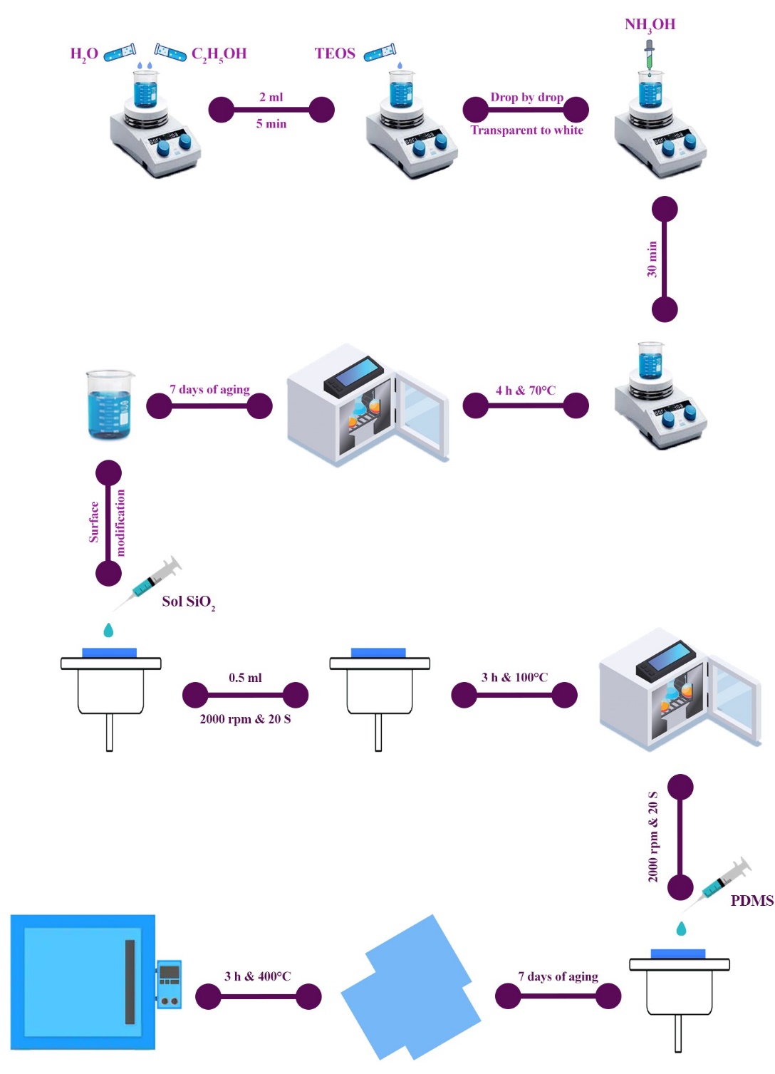
Optimized sample according to statistical data analysis, as mentioned earlier, was prepared by Stober method with TEOS as precursor, deionized water of hydrolyzing agent, solvent ethanol, ammonium hydroxide catalyst, and PDMS as a hydrophobic agent. As a result, the effect of experimental parameters on superhydrophobic coatings was investigated.
3.2.1 Optimized sample contact angle
The contact angle is the angle between the surface on which the liquid is located or the point of connection of the liquid on the surface. Static and dynamic contact angles are of its types. The method of measuring the contact angle is called the baseless droplet method. Can be used. The contact angle obtained for the optimized sample is 162 degrees (Fig. 5).
3.2.2. XRD studies
Figure 6 shows the X-ray diffraction pattern of nanoparticles prepared by the Stuber method. As shown in the figure, no diffraction peaks are observed except for broadband with a 24-degree center (JCPDS No. 0085 − 29) which represents a completely amorphous structure. But using Highscore plus software, it is shown that a small part of the sample has a crystalline structure. The marked peaks are related to hexagonal (JCPDS number 2147-080-01) and quadrilateral (JCPDS number 0430-079-01) and (JCPDS number 0513-082-01) crystal structures.
3.2.3. FTIR spectrum
Infrared spectroscopy (FT-IR) was performed at room temperature to investigate the chemical bonds created in the optimized sample. As shown in Fig. 7, the peaks of 3440 cm− 1 and 1624 cm− 1 are symmetrical tensile vibration and flexural vibration of the O-H bond, respectively, due to the incomplete density of the silanol group. The range of 400 cm− 1to 1350 cm− 1, known as the fingerprint area, indicates silicon bonds. The peak 1095 cm− 1 and 808 cm− 1 represent the symmetric and asymmetric tensile vibrations of the Si-O-Si bond and the peak 466 cm− 1 represents the flexural vibrations of the Si-O-Si. The peak of 947 cm− 1is due to the flexural vibrations of the Si-OH bond [31, 32].
3.2.4. SEM images
Scanning electron microscope images of the optimized sample at different magnifications are shown in Fig. 8. As seen in Fig. 8a, the nanostructures have spherical morphology with uniform size distribution. Particle size using image j software is approximately 250 nm. The reason for the growth of nanoparticles is due to the use of the hydrothermal method to create a suitable uneven surface on the glass surface.
Figures 8b and 8c show the scanning electron microscope image of the surface and cross-section. The roughness of the glass surface indicates a rough surface for the super-hydrophobic coating. The growth process of this superhydrophobic coating is island-layer, which is a state between layer-by-layer growth and island growth, one or more monolayers are formed and then the islands are completed. Another name for this growth process is Stransky-Kristanov. In this growth mode, a mismatched network may be formed between the coated layer and the substrate. The grain size of the thin layer that is formed on the substrate depends on the speed and temperature of the layer. The thickness of this superhydrophobic coating is reported to be 1.06 µm.
3.2.5. EDS studies
Figure 9a shows the X-ray energy diffraction spectrum for the optimal sample. As shown in the figure, the purely synthesized optimized sample is composed of silicon and oxygen elements. Figure 9b shows the X-ray diffraction spectrum from the glass surface. Due to the use of PDMS as a hydrophobic agent on the glass surface, in addition to silicon and oxygen, carbon is also seen. The gold peak seen in the figure is due to the conductivity of the surface for SEM analysis.
3.2.6. AFM images
Atomic force microscopy images of the mean square root roughness for the optimized sample are estimated in Fig. 10. As can be seen in the figure, rough surface roughness is created on the glass surface to create a super-hydrophobic coating. The maximum and minimum of these surface roughnesses were measured at 2.6 and 1.2 µm, respectively. The root means square roughness for the sample optimized by Gwyddion software was calculated to be 0.121 µm.
3.2.7. DLS analysis
As can be seen in the SEM images, the optimized sample has the same particle size distribution and DLS analysis was performed to determine the particle size distribution range. The particle size range is between 255 and 396.1 nm and, as shown in Fig. 11, the particle size distribution diagram is very narrow. The average particle size is 291.456 nm.
3.2.8. Chemical resistance test
The stability of superhydrophobic coating was investigated in three media: acidic, neutral, and alkaline. Figure 12 shows the effect of different environments on the contact angle. The superhydrophobic coating was immersed in 10 ml for 24 hours. It was then dried at room temperature. As can be seen in the figure, the play environment (pH: 13.5) has a great impact on the coating so that the drop contact angle of the super-hydrophobic range reaches the boundary between hydrophobic and hydrophilic, in which case the result can be the game environment causes corrosion of the coating and the use of this coating in play environments is not recommended. The contact angle obtained from the acidic environment (pH: 1) indicates that the coating has good resistance and this feature can be very effective in coating against acid rain. The use of deionized water is used to accurately assess the strength of the coating when in contact with water. Therefore, to prevent the effect of temperature on the coating, this test was performed at a temperature of 25 degrees. The contact angle resulting from the immersion of the coating in deionized water indicates the very good resistance of the coating in this environment.