2.1. Study Area
Hazaribagh wildlife sanctuary in Jharkhand (India) is situated covers an area of 186 km2(Fig. 1). It lies between 24°45'22” N to 24°08′20″N latitude and 85° 30'13” E to 85°21′58″E longitude. The place is home to Peafowl, Nilgai Sambar, Chital, Sloth bears, Black bears, Hyena, and Pigeons. The area experiences subtropical and humid monsoon climate characterized by hot summers (40◦C) and mild winters (4◦C).
2.3. Data pre-processing
2.3.1. For Landsat data
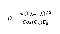
Raw satellite data required atmospheric correction for retrieving actual reflectance of objects. For this purpose, the data was automatically corrected using SAGA GIS module and to surface reflectance by Dark Object Subtraction (DOS) method. The (DOS) method presumes that over satellite image there are present features having near-zero percent reflectance (i.e., water and shadow) and this must be removed. It is calculated by below Eq. (1): (see Equation 1 in the Supplementary Files)
Where, p is the DOS corrected image and is the cosine form of solar zenith angle and E0 is the exoatmospheric solar spectral irradiance.
The Radiance (Lλ) was calculated through the below-given equation (Eq. 2)
Lλ= Bias + (Gain* DN) (2)
Where DN = Digital Number and the relflectance (Pλ) was computed by given below equation (Landsat Science User Data Handbook) (Eq. 3).
Pλ = π * Lλ * d2 / ESUNλ*Cosθ (3)
Where P and L are reflectance respectively and at-satellite spectral radiance, ESUN is mean solar exoatmospheric irradiances for a band, d is the Earth-Sun distance, and cos ø is the solar incidence angle.
2.3.2. For Sentinel 2 A data
The sentinel 2A undergoes various stages of atmospheric correction using SNAP software. The Sent2core plugin was used for transformation of Sentinel level 1 image to level 2 resembles conversion of digital number of images to surface reflectance. It helps to correct images from the presence of aerosol, ozone level distortion, type of locality, mid-latitude abnormality and topographical variations. The IdePix Sentinel MSI plugin was used for masking of land/water/ cloud in the imagery.
2.4. Computing chlorophyll content
The method of inversion of PROSAIL using SNAP software(step.esa.int/main/toolboxes/snap) is given in Fig. 3 and its illustration below.
The inputs (Sentinel2 surface reflectance 8 bands B3, B4, B5, B6, B7, B8a, B11, B12) and geometry, cos (Viewing_Zenith), cos (Sun_Zenith), cos (relative_azimuth_angle) and output (LCC) values were firstly normalized according to Eq. 4.
X* = 2*(X-XMin)/(XMax-XMin)-1 (4)
Where X* is the normalized input, X the original value, Xmin and Xmax respectively the minimum and maximum values.
Every artificial neural networking has the hidden layer and the output layer. The layer outlined by its number of neurons, which has biases, weight, and transfer function which is developed earlier and embedded in PROSAIL model.
The neurons have transfer function called tangent sigmoid transfer function (Eq. 5);
Y = Tansig(x) = 2/(1 + exp(-2x))-1 (5)
While an output layer with the transfer function is linear (y = x). It is simply involving the application of reverse function used to enter normalization given in Eq. 6.
Y = 0.5 (Y*+1) * (Ymax-Ymin) + Ymin (6)
where Y* is normalized output value (LCC) issuance from neural network, and Ymin and Ymax were calculated over the neural network training dataset.
The accuracy assessment of LCC is given in Fig. 4. It shown good Root-mean-square Deviation (RMSE) of 56.29 µg cm− 2. In case of LCC, significant correlation coefficient of 0.87 seen using artificial neural networking [28].
2.4. Vegetation indices
A vast number of vegetation indices have been used and evaluated for measuring plant physiological conditions using simulated and empirical data [29]. 9 vegetation indices were calculated using the Sentinel 2A and Landsat 8 OLI data sets, from which 7 were broadband indices while 2 vegetation indices were narrow-band indices (Table 2). The chlorophyll concentration is well predicted in the wavelengths between 400 nm to 725 nm with multiple scattering in the Near Infrared (NIR) region. Therefore, vegetation indices covered these ranges are useful in modelling LCC [39]. The wavelength of broadband vegetation indices was: Blue (436–528), Red (625–691), Green (512–620), and NIR (829–900 nm). The broad band vegetation indices were calculated using the Landsat 8 OLI. Both Broadband and narrowband indices were used to measure the relationship between LCC and the spectral response function of the forest leaf. Theoretical analyses and field studies have shown that vegetation indices are near-linearly connected to estimate biophysical variables [40]. In the present study, indices were taken because most of the biophysical measurements, for example chlorophyll estimation using remote sensing depend upon the spectral proprieties of vegetation by a semi-empirical linkage with vegetation index [41, 42]. In other means the spectral vegetation indices are popularized for retrieving chlorophyll content from reflectance factors.
Table 2
Vegetation indices used in the study
| VI | Formula | Reference |
| Infrared Percentage Vegetation Index (IPVI) |
| [30] |
| Green Vegetation Index (GVI) | (-0.2848 * TM1) + (-0.2435*TM2) + (-0.5436*TM3) +(0.7243* TM4) + (0.0840*TM5) + (-0.1800*TM7) | [31] |
| Global Environmental Monitoring Index (GEMI) |
Where:
| [32] |
| Green Atmospherically Resistance Index (GARI) |
| [33] |
| Difference Vegetation Index (DVI) | NIR-RED | [34] |
| Atmospherically Resistance Vegetation Index (ARVI) |
| [35] |
| Ratio Vegetation Index (RVI) | NIR/RED | [36] |
| Pigment Specific Simple Ratio (PSSRA) | Band 7/ Band 4 (Sentinel) | [37] |
| Normalized difference Index (ND45) | (Band5-Band4)/(Band5 + Band4) Where band 5 and 4 are sentinel 2A bands | [38] |
2.5. Modelling change detection
The forest health and stress were examined by LCC value, its decrease in value shows forest health decline and increment in plant stress. The Spatio-temporal changes of chlorophyll were computed using a grid statistics algorithm in SAGA GIS. Then, the scatter plot matrix was used to find the relationship of LCCtime to LCCtime+1 using Geoda software (https://spatial.uchicago.edu). Time was the year taken for temporal variation of Chlorophyll.