2.1. Study area
Guangdong Province and Guangxi Zhuang Autonomous Region are located on the southern coast of China and are commonly known as the Guangdong and Guangxi regions. Guangdong and Guangxi are rapidly growing and densely populated urban areas in China, and they share significant similarities in location, size, climate, topography, and resources. The geographical location and administrative division of the study area were shown in Fig. 1.
Guangdong Province has a central subtropical, southern subtropical and tropical climate from north to south, respectively. The northern half of Guangxi Zhuang Autonomous Region has a central subtropical climate, while the southern half has a southern subtropical climate. Guangdong and Guangxi regions are rich in light, heat and water resources, and rain and heat are synchronized, with precipitation mainly concentrated in April-September (Baidu Encyclopedia 2022).
Affected by the monsoon climate, Guangdong and Guangxi are the regions with the maximum distribution of summer precipitation and inter-annual variability in China. The annual precipitation in Guangdong Province ranged from 1179.6 mm to 2320.9 mm (Guangdong Meteorological Bureau 2022), and that in Guangxi Zhuang Autonomous Region ranged from 1210.4 mm to 2190.9 mm (Meng J 2019). At the same time, there are also problems such as low altitude, aging pipeline network and imperfect flood control projects in Guangdong and Guangxi (Zhang and Tang 2020; Zhao and Zhang 2017). Therefore, during the period of concentrated rainfall every year, the Guangdong and Guangxi regions are faced with severe waterlogging risk.
2.2. Data collection
The remote sensing images, DEM data and administrative boundaries of the Guangdong and Guangxi regions in 2020 were obtained through the open source map software-LocaSpace Viewer. Weibo texts were chosen as the data source. Based on the open interface of Weibo platform, the index phrases were formed by keywords such as "flood", "waterlogging" and "trapped", and obtained the original sign-in data of urban waterlogging disasters in Guangdong and Guangxi from June 1, 2020 to September 30, 2020. Through manual screening, duplicate data, pictures, videos and other data are deleted, and 6125 pieces of valid text data were finally obtained. The number of Weibo texts for different dates and different cities are shown in Fig. 2 and Fig. 3.
2.3. Methods
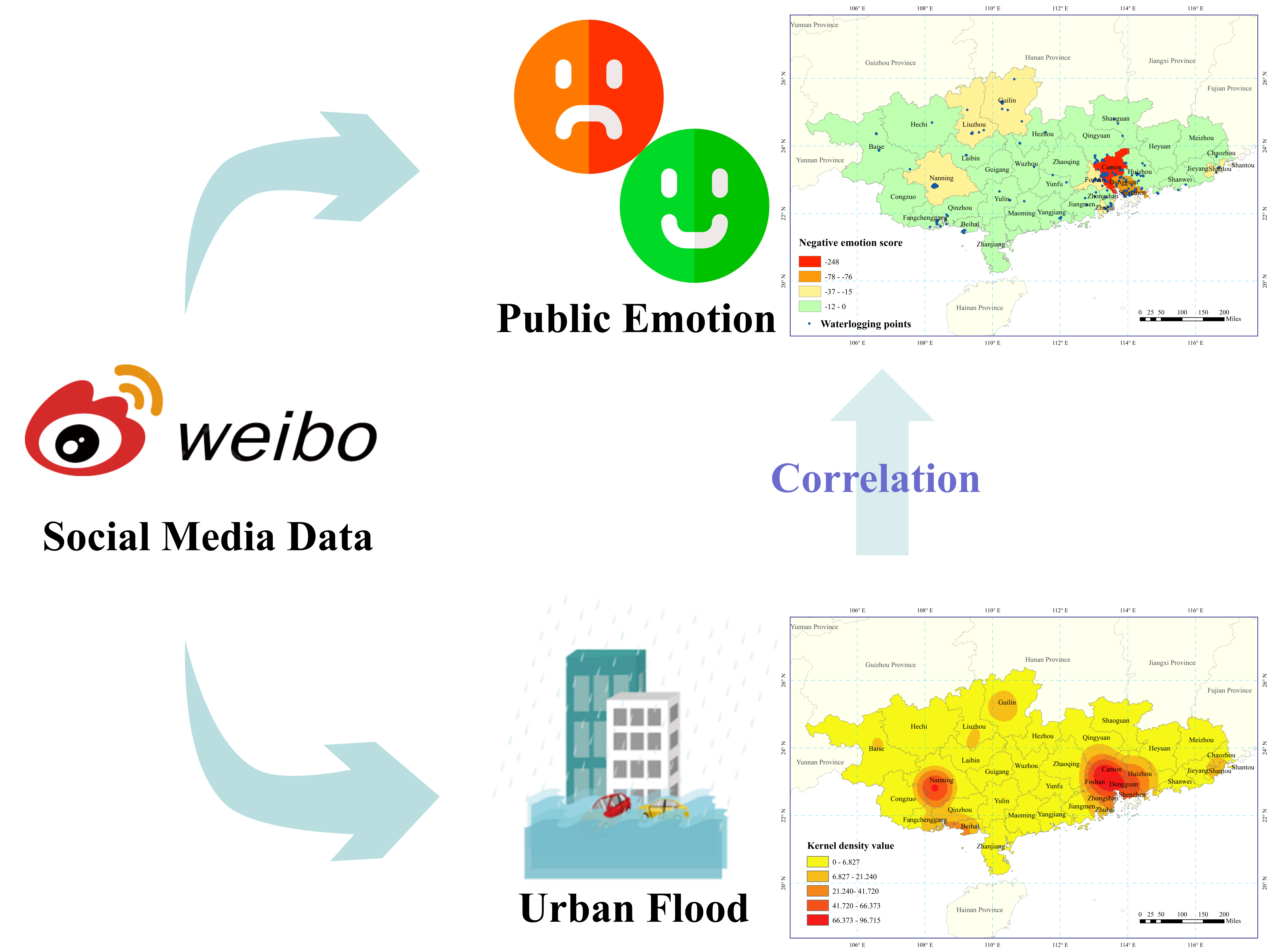
The framework and approach used in this study was schematically depicted in Fig. 4, which mainly contained three parts: Weibo database construction, analysis of disaster situation and public emotion, correlation analysis between disaster situation and public emotion.
2.3.1. Weibo database construction
Firstly, Web Scraper was used to obtain flood-related Weibo texts between June 1, 2020 and September 30, 2020. Web Scraper is a Google Chrome-based crawler tool that is free and does not require a high level of programming from the user (Sspai Web 2020). After that, duplicate data, images and videos were removed through manual screening. In this way, a database of flood-themed Weibo texts was obtained.
2.3.2. Analysis of disaster situation
In order to extract useful information from Weibo texts, the collected texts were first divided into words using “jieba” (Chen and Song 2020). “jieba” (Chinese for “to stutter”) Chinese text segmentation is a Python Chinese word segmentation module. The functions of “jieba” include text segmentation, keyword extraction, lexical annotation and word position query. After obtaining the results of text segmentation, the analysis of the disaster situation and public emotion can be launched (GitHub Web 2020).
In the analysis of the disaster, Baidu Maps was used to obtain the coordinates of the location where the waterlogging occurred in Weibo texts. The coordinates of these waterlogging points were represented in ArcGIS, and then the spatial distribution characteristics of waterlogging were explored by the Kernel Density Analysis (Allen et al. 2021). Kernel Density Analysis is a method used to calculate the unit density of the measured values of point and line elements within a specified neighborhood. It visualizes the distribution of discrete measurements over a continuous area. The result of Kernel Density Analysis is a smooth surface with large intermediate values and small peripheral values, and the raster value is the unit density. The Kernel Density Analysis uses the following function.
$$D=\frac{{3(1-{scale}^{2})}^{2}}{\pi {r}^{2}}$$
In the above formula, r is the lookup radius, scale is the ratio of the distance from the grid center point to the point or line object to the lookup radius. For a point object, the volume of the space enclosed by its kernel density surface and the plane below approximates the measurement at this point. For a line object, the volume of the space enclosed by the kernel density surface and the plane below is approximated by the product of the measurement of this line and the length of the line (IDesktop Web 2022).
2.3.3. Analysis of public emotion
Baidu Natural Language Processing was used to analyze public emotion (Zhang and Gan 2020). Baidu Natural Language Processing is a tool to analyze the emotional tendencies of Chinese, which is built on deep learning technology and Baidu big data. Baidu Natural Language Processing can automatically determine the sentiment polarity category of the text, including positive, negative and neutral, and give the corresponding confidence level. The emotion polarity category of each Weibo text was determined, and then positive, negative and neutral were expressed as 1, -1 and 0, respectively, to quantify the public emotional score (Wang et al. 2020).
Based on the text segmentation results, the TF-IDF formula was used for semantic-based classification of Weibo texts (Sarirete A 2022). TF-IDF is a statistical method to assess the importance of a word for a document set or one of the documents in a corpus. The importance of a word increases positively with its number of occurrences in a document, but decreases inversely with its frequency in a corpus.
$$t{f}_{i,j}=\frac{{n}_{i,j}}{{\sum }_{k}{n}_{k,j}}$$
In the above formula, \({f}_{i,j}\) represents the number of times that item \({t}_{i}\) appears in Weibo \(j\), the numerator is the number of times the word appears in the text, and the denominator is the sum of the number of times that all words appear in the text (Natural Language Processing Column 2022).
Combining existing studies (Wu et al. 2018) and the contents of the collected microblog texts, the feature items after calculating the weights were divided into three categories: disaster descriptions, pre-disaster warnings and news reports, and emotional expressions and related thoughts.
2.3.4. Correlation analysis between disaster situation and public emotion
The data of waterlogging points and negative emotion scores of each city were tested to be in line with normal distribution. Pearson correlation analysis and partial correlations analysis were used to analyze the correlation between waterlogging and negative public emotion (Ates and Guran 2021). Pearson correlation analysis is a method proposed by British statistician Pearson and is widely used to measure the degree of correlation between two variables, its result is represented by the correlation coefficient \(r\).
$${r}_{X,Y}=\frac{n\sum XY-\sum X\sum Y}{\sqrt{\left[N\sum {X}^{2}-{\left(\sum X\right)}^{2}\right]\left[N\sum {Y}^{2}-{\left(\sum Y\right)}^{2}\right]}}$$
In the formula, \(n\) is the sample size, \(X\) and \(Y\) are the observed values of the research variables. Generally defined, if \(r\) >0, it can be concluded that the two variables are positively correlated, otherwise, it is negatively correlated. The larger the absolute value of \(r\), the stronger the correlation between the two variables (Machine Learning and Artificial Intelligence Column 2021).
Partial Correlations Analysis is the process of eliminating the effect of the third variable when two variables are simultaneously correlated with a third variable, and analyzing only the degree of correlation between the two variables to be explored. In analyzing the correlation between two variables X and Y, with Z as the control variable, the partial correlation coefficient between X and Y is defined as \({r}_{xy\left(z\right)}\).
$${r}_{xy\left(z\right)}=\frac{{r}_{xy}-{r}_{xz}{r}_{yz}}{\sqrt{1-{r}_{xz}^{2}}\sqrt{1-{r}_{yz}^{2}}}$$
In the formula, \({r}_{xy}\) is the correlation coefficient of x and y, \({r}_{xz}\) is the correlation coefficient of x and z, \({r}_{yz}\) is the correlation coefficient of y and z. The larger the absolute value of \({r}_{xy\left(z\right)}\), the stronger the correlation between x and y (Mengte Web 2022).
2.3.5. Natural Breaks Classification (Jenks)
There are some natural turning points and breakpoints between any series of numbers, and these natural breakpoints are statistically significant, and with these turning points the objects of study can be divided into clusters of similar nature. Therefore, the natural breakpoints themselves are good bounds for grading (GIS Column 2016). Natural breakpoints were used in this study to classify the kernel density of waterlogging points and emotion scores.