2.1 Source of the data
The source of the data in this study is the 2011 Ethiopia Demographic and Health Survey (EDHS). The 2011 EDHS was conducted by the Central Statistics Agency (CSA) with support from the ministry of Health. The analysis presented in this study on under-five mortality was based on the 10,475 women aged 15–49 years. During the analysis stage, Statistical Package for Social Science (SPSS) version 16, South Texas Art Therapy Association (STATA) version 12 and Microsoft-Excel were used as tools of analysis.
2.2 Variables in the study
The dependent variable for this study is the number of deaths of under- five deaths per mother. Based on the [15] determinants of childhood morbidity and mortality framework for developing countries, experiences from the available similar studies and available data on the subject, the main predictors explored for under-five mortality have been grouped into demographic, socioeconomic and environmental factors. The demographic factors for this studies are mother’s age at the firth birth, mother’s currently breastfeeding and mother’s marital status. The socioeconomic factors are mother’s level of education, mother currently working, region and household’s wealth index. The environmental factors are Source of drinking water and Toilet facility.
2.3 Methods of data analysis
In this study, the variable of interest is a count variable. When the response or dependent variable is a count (which can take on non-negative integer values (0, 1, 2, …), it is appropriate to use non- linear models based on non- normal distribution to describe the relationship between the response variable and a set of predictor variables. For count data, the standard framework for explaining the relationship between the outcome variable and a set of explanatory variables includes the Poisson and negative binomial regression models. Unlike linear regression, count data regression models have counts as the response variable that can take only nonnegative integer values. The two most popular models for count data are the Poisson model and the negative binomial model.
2.3.1 Poisson regression model
This regression model is a popular and simple regression model for count data. It assumes a Poisson distribution, characterized by a positive skewed and a variance equals the mean. Poisson regression analysis is a technique which allows to model dependent variables that describe count data [3]. According to [19], the apparent simplicity of Poisson comes with two restrictive assumptions. First, the variance and mean of the count variable are assumed to be equal. The other restrictive assumption of Poisson models is that occurrences of the event are assumed to be independent of each other.
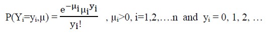
Let Yi represent counts of events occurring in a given time or exposure periods with rate µi. Yi are Poisson random variables which the p.m.f. is characterized by
[Due to technical limitations, this equation is only available as a download in the supplemental files section.]
where, yi denotes the value of an event count outcome variable occurring in a given time or exposure periods with mean parameterµi.
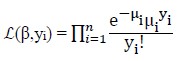
The likelihood function of the Poisson model based on a sample of n independent observations is given by
[Due to technical limitations, this equation is only available as a download in the supplemental files section.]
The log-likelihood function is
[Due to technical limitations, this equation is only available as a download in the supplemental files section.]
The likelihood equation for estimating the parameter is obtained by taking the partial derivations of the log-likelihood function and setting them equal to zero.
There are two basic criteria commonly used to check the presence of overdispersion:
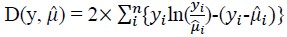
1. Deviance, D(y, μ), is given by
[Due to technical limitations, this equation is only available as a download in the supplemental files section.]
where, y is the number of events, n is the number of observations and μ̂i is the fitted Poisson mean.
2. Pearson chi-square test,x2 is also given by
[Due to technical limitations, this equation is only available as a download in the supplemental files section.]
Another way of checking the presence of over-dispersion is a statistical test of the hypothesis:
H0: α = 0 vs H1: α > 0.
If P-value of LRTα < α (level of significant), which is an indicated of over-dispersion is present; negative binomial is preferred. The negative binomial regression model is more appropriate for over-dispersed data because it relaxes the constraints of equal mean and variance.
In the general Poisson regression model, we think of μi as the expected number of under five-child death from the ith mother and the total number children ever born from the ith mother is Ni. This means parameter will depend on the population size and the total number of children ever born from the individual mother. Thus the distribution of Yi can be written as:
𝐘𝐢~𝐩𝐨𝐢𝐬𝐬𝐨𝐧 (𝐍𝐢𝛍𝐢)
Where, 𝐍𝐢 is the total fertility rate of ith mother and 𝛍𝐢 = (𝐗𝐢T𝛃)
The logarithm of the children ever born is introduced in the regression model as an offset variable. By including ιn[children ever born] as offset in the equation, it is differentiated from other coefficients in the regression model by being carried through as a constant and forced to have a coefficient of one [9].
2.3.2 Negative binomial regression model
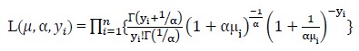
This model is used when count data are overdispersed (i.e when the variance exceeds the mean). Overdisprsion, caused by heterogeneity or an excess number of zeros (or both) to some degree is inherent to most Poisson data. By introducing a random component into the conditional mean, the negative binomial regression model addresses the issue of over-dispersion. However, it equally models both zero and nonzero counts, which might result in a poor fit for data with excessive number of zeros. Therefore, it is always necessary to check the proportion of zero counts before developing a negative binomial regression model. We used the likelihood ratio test to determine the more appropriate model between the Poisson regression and negative binomial regression. [11] used negative binomial regression to model over dispersed Poisson data.. The NB regression model is
[Due to technical limitations, this equation is only available as a download in the supplemental files section.]
with mean and variance are given by
E(Yi) = μi = exp(xiTβ) and Var(Yi) = μi(1+αμi)
where, α shows the level of overdispersion and Γ(.) is the gamma function.
The likelihood function of the NB model based on a sample of n independent observations is given by
[Due to technical limitations, this equation is only available as a download in the supplemental files section.]
The log-likelihood function l of NB regression model is
[Due to technical limitations, this equation is only available as a download in the supplemental files section.]
For estimating regression coefficients β and dispersion parameter α, the Newton-Raphson iteration procedure is applied like Poisson model.
2.3.3 Zero- inflated model
In some cases, excess zeros exist in count data and considered as a result of over-dispersion. In such a case, the NB model cannot be used to handle the over-dispersion which is due to the high amount of zeros. To do this, zero-inflation (ZI) can be alternatively used.
2.3.3.1 Zero- inflated Poisson regression model
The Zero-inflated Poisson regression study the relationship between dependent and independent variable(s) when there are many zeros value in the dependent variable, where the relationship is the mixture between Poisson model and Logistic model. Zero-inflated Poisson Regression also provides a flexible way of modeling zero counts and an attractive interpretation.
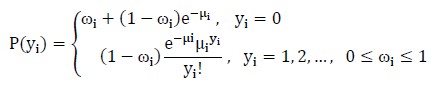
The ZIP regression model is [14],
[Due to technical limitations, this equation is only available as a download in the supplemental files section.]
where, Yi~ZIP (μi,ωi). The mean and variance of ZIP are given by
E(Yi) = (1-ωi)μi and Var(Yi) = E(Yi)( (1+ωiμi)
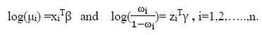
The parameters μi and ωi can be obtained by using the link functions,
[Due to technical limitations, this equation is only available as a download in the supplemental files section.]
where, xiT and ZiT are covariate matrices, β and γ are the (p+1)×1 and (q+1)×1 unknown parameter vectors, respectively. The log-likelihood function of ZIP model is given by
[Due to technical limitations, this equation is only available as a download in the supplemental files section.]
where, I (.) is the indicator function for the specified event, i.e. equal to 1 if the event is true and 0 otherwise.
To obtain the parameter estimates of ZIP regression models, β ̂and γ̂, the Newton-Raphson method can be used.
2.3.3.2 Zero-inflated negative binomial regression model
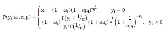
Zero-Inflated Negative Binomial (ZINB) regression is one of the methods used in troubleshooting overdispersion due to excessive zero values in the response variable (excess zeros). This model provides a way of modeling the excess number of zeros (with respect to a Poisson distribution or negative binomial distribution) in addition to allow for count data that are skewed and overdispresed. We used the vuong test, likelihood ratio based test, to compare the zero inflated negative binomial model with negative binomial regression model. A significant z-test indicates that the zero inflated models are preferred. We consider 𝑌𝑖 as a ZINB distribution. Specifically, we consider the distribution. [10] used the zero-inflated negative binomial (ZINB) regression to model overdispersed data with an excess of zeros. This regression model was given by
[Due to technical limitations, this equation is only available as a download in the supplemental files section.]
where, µi is the mean of the underlying negative binomial distribution, α >0is the over dispersion parameter and is assumed not to depend on covariates and 0 ≤ 𝜔𝑖 ≤1. Also the parameters 𝜇𝑖 and 𝜔𝑖 depend on vectors of covariates 𝑥𝑖 and 𝑧𝑖, respectively.
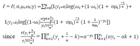
The log-likelihood function l = l(α,µi,ωi;y), for the ZINB model is given below.
[Due to technical limitations, this equation is only available as a download in the supplemental files section.]
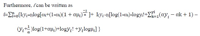
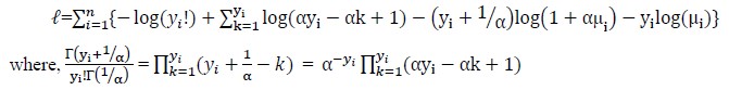
Furthermore, l can be written as
[Due to technical limitations, this equation is only available as a download in the supplemental files section.]
Newton-Raphson iteration procedure can be used for estimating the parameter of ZINB regression models.
2.4 Goodness of fit tests
2.4.1 Likelihood Ratio test
The Likelihood ratio test is a test of a null hypothesis H0 against an alternative H1 based on the ratio of two log-likelihood functions. The likelihood ratio test is a test of the overall model. The overall test statistic for likelihood ratio test is given as:
[Due to technical limitations, this equation is only available as a download in the supplemental files section.]
This statistic is called the likelihood-ratio test statistic.
Where: lnull is the log-likelihood of the null model and lk is the log-likelihood of the model comprising k predictors, p is number of parameters and xp–12 is a chi-square distribution with p–1 degree of freedom. If the test statistics exceeds the critical value, the null hypothesis is rejected. That means the overall model is significant. In this study, to compare Poisson and NB regression models and also ZIP with ZINB regression models, we used significance of dispersion parameter and likelihood ratio (LR) test as criterions. The statistic of likelihood ratio test for α is given by the following equation: LRTα = –2(LL1—LL2)
This statistic has a Chi-squared distribution with 1 degrees of freedom and LL is log-likelihood. If the statistic is greater than the critical value then, the model 2 is better than the model 1.
2.4.2 Vuong Test
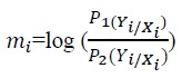
The Vuong test is a non-nested test that is based on a comparison of the predicted probabilities of two models that do not nest [21]. That means vuong test statistics are needed to provide the appropriateness of zero-inflated models against the standard count models. For testing the relevance of using zero-inflated models versus Poisson and NB regression models, the Vuong statistic is used. Let’s define [Due to technical limitations, this equation is only available as a download in the supplemental files section.]
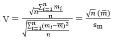
where, P1(Yi/Xi) and P2(Yi/Xi) are probability mass functions of zero-inflated and Poisson or NB models, respectively. In general, PN(Yi/Xi) is the predicted probability of observed count for case i from model N, then the Vuong test statistic is simply the average log-likelihood ratio suitably normalized. The test statistic is [Due to technical limitations, this equation is only available as a download in the supplemental files section.]
Where, m̅ is mean of mi, sm standard deviation and n sample size.
The hypotheses of the Vuong test are:
Ho: E[mi] = 0
The null hypothesis of the test is that the two models are equivalent. Vuong showed that asymptotically, V has a standard normal distribution. As Vuong notes, the test is directional [21].
- If V > Zα/2, the first model is preferred.
- If V < -Zα/2, the second model is preferred.
- If | V | < Zα/2, none of the models are preferred.
2.4.3 AIC and BIC
AIC and BIC are goodness of criteria used for model selection. The likelihood ratio test was used to compare the Poisson model and NB model. Many Monte-Carlo simulations indicate that the BIC and AIC selection criteria need to be used together [4] and [23]. The model with smallest value of AIC or of BIC is preferable. Selecting an appropriate model can be used a standard likelihood information criteria, for example, Akaike information criteria [2] or Baysians information criteria [18] abbreviated by AIC and BIC, respectively, Where
AIC = –2 log likelihood+ 2k
BIC = –2 log likelihood +k ln(n)
where, k = number of parameters and n = number of observations.