Data acquisition
Two long-read cDNA and dRNA sequencing datasets were downloaded and analyzed during the study. (1) The human cDNA and dRNA sequencing FASTQ reads of the Nanopore WGS Consortium (https://github.com/nanopore-wgs-consortium/NA12878/blob/master/RNA.md) were generated by extracting RNA from the GM12878 human cell line (Ceph/Utah pedigree) and sequenced on MinION flow cells (FLO-MIN106) using R9.4 chemistry (SQK-RNA001 and SQK-LSK108 kits) [22]. This dataset will be referred to as the human dataset. (2) Previously published [23, 33] data of the lytic HCMV transcriptome were downloaded from the European Nucleotide Archive, from the accession numbers PRJEB22072 (https://www.ebi.ac.uk/ena/data/view/PRJEB22072) and PRJEB25680 (https://www.ebi.ac.uk/ena/data/view/PRJEB25680). RNA was isolated from HCMV-infected (strain Towne, ATCC VR-977) human embryonic fibroblast cells (MRC-5, ATCC CCL-171) and sequenced on the RSII and Sequel platforms of Pacific Biosciences using the Iso-Seq library preparation protocol and on the MinION platform using the SQK-RNA001 and SQK-LSK108 kits and another cDNA library was prepared combining the SQK-LSK108 and the TeloPrime Full-Length cDNA Amplification Kit (Lexogen) to select for capped RNA molecules. In this latter experiment, the TeloPrime kits own enzymes were used for poly(A)-selection. This dataset containing results from five sequencing libraries (RSII and Sequel Iso-Seq libraries, MinION cDNA, cap-selected MinION cDNA and MinION dRNA libraries) is referred to in the text as the HCMV dataset.
Mapping and read processing
The computational pipeline of the study is summarized in Additional file 2Figure S2. The processing steps for the human and HCMV data were the same. The reads were mapped using minimap2 [34] to the human genome (hg19) and to the HCMV strain Towne varS genome (LT907985). Reads from the HCMV dataset were only mapped to the viral genome, reads from the viral infected host were not used. The mapper settings were “-ax splice -Y -C5” for the cDNA and “-ax splice -uf -k14” for the dRNA sequencing reads. Coverage and dRNA read endings were determined using bedtools [35]. As dRNA sequencing does not accurately sequence the terminal poly(A) tail of the reads, every dRNA read ending was counted. A genomic locus was confirmed as a poly(A) site confirmed by dRNA sequencing, if at least 0.5% of the overlapping dRNA reads ended in the 21-nt window (10nt upstream + the locus + 10nt downstream = 21nt) around the locus.
Identifying potential poly(A) sites in the cDNA sequencing data
The LoRTIA toolkit (https://github.com/zsolt-balazs/LoRTIA) was used to identify potential poly(A) sites in the cDNA sequencing data. A genomic locus was considered a potential poly(A) site when at least two reads and at least 0.1% of the overlapping reads ended at a given nucleotide. In a 21-nt window, the genomic position with the highest number of poly(A)+ reads was selected as the potential poly(A) site. The separate experiments of the HCMV dataset were analyzed separately and the results were joined to create the list of potential HCMV poly(A) sites. The LoRTIA toolkit was also used to mark reads which ended in A-rich genomic regions (three or more consecutive As as potentially artefactual reads). When characterizing high confidence calls only the sites where more than ten reads ended in a 21-nt window around the locus were analyzed.
Defining A-rich regions
We have deployed a slightly different definition of A-rich regions than it is commonly used in the literature. A common approach is to count the number of consecutive As in a region surrounding the poly(A) site. Another method is to count the number As in a given, often 20-nt-long window (because 20nt is the primer length). Instead, we iterated the 20nt upstream of a potential poly(A) site and incremented a counter each time an A was iterated, all the other nucleotides were counted as -1. If the counter reached -1, the iteration was halted and the highest count was regarded as the A-count of the region (Additional file 2 Figure S2). This method of defining A-rich regions combines the strengths of the previously described methods. It (1) gives more weight to As close to the polyA-site, which are more likely to contribute to the generation of artefacts. However, (2) it still considers the broader environment of the site, not just consecutive stretches of As.
Filtering out template-switching (TS) artefacts
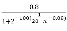
The potential poly(A) sites which were not at A-rich loci, were accepted by our script as transcriptional end sites. The potential poly(A) sites at A-rich loci were accepted as TES if the number of reads in a 21-nt window around that loci contained either more reads which ended in a non-A-rich region than reads which ended in an A-rich region or a proportion of overlapping reads greater than (see Equation in the Supplementary Files) where n is the number of As in the A-rich region. The potential poly(A) sites which did not meet these requirements were classified as TS artefacts. The genomic loci which contained at least 100 times more 5’-ends from the opposite strand than 3’-ends were also classified as artefactual poly(A) sites. The sites which were classified as TS artefacts, but were no further than 50nt away from sites that were classified as TES, were excluded from comparisons and sequence analyses in order to prevent the characteristics of the TES to interfere with the characteristics of TS artefacts (e.g. a polyadenylation signal that is upstream of a TES could also be upstream of a TS artefact, similarly, a direct RNA read ending in the proximity of a TES could also fall into the 21-nt window of an artefactual site).
Detecting polyadenylation signals
The 12 most commonly utilized human PAS [27] were searched for in the region 40nt upstream of each potential poly(A) site. Only exact matches were accepted. If the sequence upstream of a potential poly(A) site contained multiple PAS sequences, the most common PAS was assigned to the site.
Measuring poly(A) tail length
The length of the sequenced poly(A) tail of the cDNA reads was measured for each read that contained a poly(A) tail recognized by the LoRTIA toolkit. The sequence containing the 3’-terminal 30nt of the mapped part of the read and the first 150nt of the 3’-terminal soft clipped (unmapped) part of the read was aligned to a stretch of 180 As using the Smith-Waterman algorithm (match score: +2, mismatch score: -3, gap opening score: -3, gap extension score: -3). The number of As in the best local alignment was counted as the length of the poly(A) tail. Measuring the poly(A) tail length this way may overestimate poly(A) tail length in A-rich regions, however it allows for a more accurate measurement in error prone reads.
Comparison with the PolyA_DB
The PolyA_DB data [36] (Release 3.2) containing polya(A) sites which were identified using the 3’READS+ method were downloaded from the projects webpage (http://exon.umdnj.edu/polya_db/v3/misc/download.php). Potential poly(A) sites were considered confirmed by the PolyA_DB dataset if the database contained poly(A) sites in the 21-nt window of the potential poly(A) sites.
Filtering using SQANTI
The potential pA sites in the human sample were filtered using SQANTI [25], a quality control software frequently used in long-read transcriptomics. The tool was run with the default settings of filtering out pA sites with higher than 80% A-content in the upstream 20 nucleotides.