Phengaris alcon genome sequencing and annotation
We collected caterpillars of Phengaris alcon by screening host plants (G. pneumonanthe) for the presence of eggs on the 31st of August 2021 near Zürich, Switzerland (8.5007°E, 47.2847°N). Plant material was immediately frozen and caterpillars subsequently dissected out. DNA was extracted from a whole caterpillar using a standard phenol/chloroform extraction method (Green & Sambrook 2017). We then sequenced its DNA on a PacBio Sequel II platform (Pacific Biosystems, Menlo Park, CA, USA) using one PacBio SMRT cell. Sequencing and library preparation followed the PacBio Low DNA Input Library protocol and was done by the Functional Genomic Centre Zürich (Zürich, Switzerland).
All obtained hifi reads were used for assembly with hifiasm 0.16.0 using standard parameters (Cheng et al. 2021). To identify contigs of non-lepidopteran origin, we compared each contig against the NCBI nucleotide collection using Blast + 2.9.0 (Camacho et al. 2009). A total of 28 contigs, accounting for 0.6% of the initial assembly length, were subsequently filtered out. Out of these filtered contigs, one contig represented the complete Wolbachia genome, which we kept as a separate assembly. We estimated the completeness of our filtered P. alcon genome with the Busco pipeline 5.1.2 (Manni et al. 2021), which was performed against the lepidoptera_odb10 database containing 5286 BUSCO groups of highly conserved single copy orthologs. We next identified repeats using RepeatMasker 4.1.3 (www.repeatmasker.org) and performed gene annotation with Braker2 (Brůna et al. 2021) on the soft masked assembly. For the latter, we took the BUSCO odb10_arthropoda protein database as a reference (Kriventseva et al. 2019). We only kept gene predictions showing support by hints, using the script selectSupportedSubsets.py of the Braker2 pipeline.
Genomics of the Swiss Phengaris alcon complex
We collected 35 specimens of the Phengaris alcon complex between 2016 and 2021, covering the three ecotypes, i.e., the low elevation P. alcon, the mid elevation and high elevation Alpine P. rebeli, respectively (Table S2). In some cases, whole bodies were collected, while in other cases, only one leg or a caterpillar was obtained. Tissue was stored in absolute ethanol prior to DNA extraction, for which we used the Qiagen Blood & Tissue Kit (Qiagen AG, Hombrechtikon, Switzerland) following the manufacturer’s protocol. Because DNA yield was low for legs and caterpillars, we performed whole genome amplifications with the Qiagen REPLI-g Kit. Paired-end sequencing libraries were prepared at the Department of Biosystems Science and Engineering (DBSSE) of ETH Zürich in Basel, followed by whole-genome sequencing (WGS) on an Illumina NovaSeq 6000. Samples were sequenced on two lanes of S4 flow cells.
We processed demultiplexed raw sequence reads as follows: First, we trimmed poly-G tails with fastp (Chen et al. 2018) and mapped all retained reads against our Phengaris alcon reference assembly, using bwa v0.7.17 (Li 2013). We then employed SAMtools v.1.13 (Li et al. 2009) to remove unmapped, unpaired, or duplicated reads. We called variants for all individuals combined with BCFtools v.1.12 (Danecek & McCarthy 2017). Finally we used VCFtools 0.1.16 (Danecek et al. 2011) to remove i.) non-biallelic SNPs, ii.) indels, iii.) SNPs with genotype quality score < 30, iv.) SNPs with more than 20% missing data, v.) SNPs with minor allele frequencies (MAF) < 0.03, and vii.) SNPs with depths < 6 or > 40. This resulted in a dataset containing 494’213 SNPs. Six individuals were subsequently filtered out due to high levels of missingness (Table S2), resulting in 29 individuals for analyses.
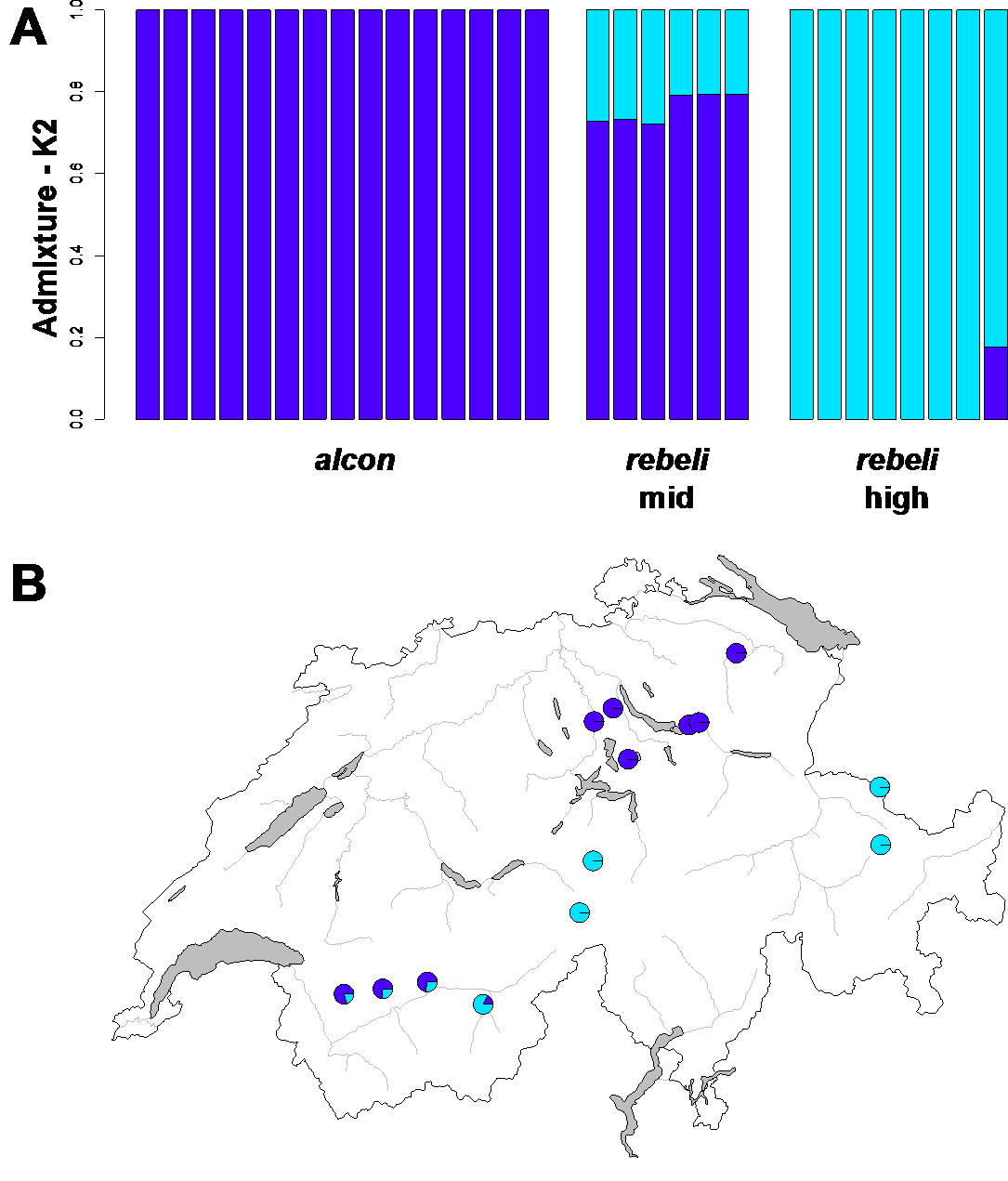
We inferred population structure in a first step with Admixture 1.3.0, which implements a likelihood approach to estimate ancestry (Patterson et al. 2012). We ran Admixture first across all individuals, varying the values for K, i.e., the number of assumed populations, from 1 to 10 and performed a cross-validation test to determine the optimal value of K. To remove effects driven by increased linkage disequilibrium, we only considered SNP sites that were at least 1’000 bps away from each other for Admixture (NSNPs= 111’414). In a second step we used a principal component (PC) analysis as implemented in PLINK 1.90b (Chang et al. 2015) to visualize the genetic relationship among individuals. Subsequent statistical analyses on the resulting PC scores were done using linear models in R 4.1.1 (R Core Team 2021).
To infer the phylogenomic structure across all retained specimens, we first used RAxML 8.2.11 (Stamatakis 2014), implementing a generalised time-reversible (GTR) model with optimised substitution rates and a gamma model of rate heterogeneity. We further applied an ascertainment bias correction to account for the fact that we only used polymorphic SNP positions with the ASC_GTRGAMMA function implemented in RAxML. Statistical support was assessed using 1’000 bootstrap replicates followed by a thorough maximum likelihood search.
Next, we estimated the level of pairwise genetic differentiation (FST) among our three Phengaris ecotypes using VCFtools, pooling individuals from across the distribution range for P. alcon, P. rebeli mid elevation and P. rebeli high elevation, respectively. For each comparison, we defined regions of accentuated genetic divergence as 10’000 bps windows for which the average FST > 0.95 and contained more than two SNPs. We subsequently extracted the gene sequence for these regions and used NCBI blastx (Boratyn et al. 2013) to identify their correspondence to other Lepidoptera.
Lastly, we assessed the potential for gene flow among our sampled individuals. First by reconstructing a network using SplitsTree 5 with a GTR model (Huson & Bryant 2006) using all available SNPs. Secondly, we estimated recent migration rates among our three ecotypes with BA3-SNPs 3.0.4 (Mussmann et al. 2019), a modification of BayesAss (Wilson & Rannala 2003) that allows the handling of large SNP datasets. For this, we assessed the optimal mixing parameters for migration rates (deltaM = 0.2688), allele frequencies (delta = 0.5500), and inbreeding coefficients (deltaF = 0.0188) by running ten repetitions in BA3-SNP-autotune 3.0.4 as recommended by Mussmann et al. (2019). Subsequently, BA3-SNPs was run with the predefined mixing parameters for 50 million generations, sampling every 100th generation. Because BA3-SNPs is computationally intensive for very large datasets (Mussmann et al. 2019), we had to run this analysis on a thinned dataset, using only SNPs that were at least 10’000 bps apart (NSNPs=30’320).
The biogeographic context of the Swiss Phengaris alcon complex
To set our Swiss samples into a broader biogeographic context, we aligned the dataset of Koubínová et al. (2017) comprising single-end RAD sequences for 25 P. alcon and one P. rebeli specimen (designated as “alpine” ecotype in Koubínová et al. (2017)) from outside Switzerland against our reference assembly. Alignment, SNP calling and filtering were done for the WGS dataset, and one P. alcon specimen from the Italian Alps had to be removed due to missingness. We subsequently extracted the overlapping SNPs between both datasets (N = 883) for our subsequent analyses. As for the Swiss specimens, we inferred the phylogenomic structure across all individuals with RAxML and visualized the population structure with a PCA in PLINK.
Wolbachia
We annotated the obtained Wolbachia assembly with the Rapid Annotation using Subsystem Technology (Rast) web service version 2.0 (Aziz et al. 2008). To test if P. alcon and P. rebeli also have different Wolbachia strains, we aligned all our genomic data against our Wolbachia assembly. Alignment, variant calling and filtering were performed as outlined above. We then established the relationship of Wolbachia among our Phengaris host individuals using RAxML with 1’000 bootstrap replicates.