Following the deployment of the Learning Management System (LMS) platform in higher educational institutions in Ethiopia, a massive amount of potentially helpful but as-yet untapped educational data has been generated. Despite the fact that the data is powerful enough to contribute to reducing student dropout rates through the application of modern educational data mining techniques such as machine learning, it has not been successfully employed to tackle student academic performance problems in higher education institutions(HEIs). As a result, a machine learning model was proposed based on data from three semesters of undergraduate students at Bule Hora University. To predict students' academic achievement, five machine learning methods (SVM, Random Forest, KNN, Gradient Boosting, and Decision Tree) were used. The Decision Tree model outperformed other models with a promising result of 97.3% on test accuracy and was selected as a proposed model. Moreover, our findings suggest that academic factors (entrance result, study time, attendance, and Internet access) and socio-demographic factors (age, gender, father job, mother job, family size, and address) had a greater impact on students' academic success. However, the academic performance of students was less affected by additional features like extra classes, another job, and guidance and counselling. Moreover, we are working on improving the accuracy of the proposed model. In this study, the student entrance result is the only variable used from the pre-university data. However, a CGPA result is not sufficient to qualify a student. Therefore, in the future, the exit exam results of the students will be incorporated.
Research Article
Multi-Category Prediction of Students’ Academic Performance Using Machine Learning: For Students Joining Higher Educational Institutions in Ethiopia
https://doi.org/10.21203/rs.3.rs-3342736/v1
This work is licensed under a CC BY 4.0 License
Version 1
posted
You are reading this latest preprint version
Learning Management System (LMS)
Multi-Category
Machine Learning
Higher Educational Institutions (HEIs)
Students’ Academic Performance
Finer Grained Level
Educational Data Mining (EDM)
Recently, large amounts of data on student academic performance have been produced due to the implementation of the learning management system (LMS) platform in higher educational institutions (HEI) [1] [2] [3]. Therefore, the potential to extract valuable knowledge and insights from educational data has gained momentum. The extracted knowledge has the potential to assist decision-makers if tapped properly. If extracted properly, this knowledge has the potential to significantly impact students’ learning experiences, learning outcomes, efficiency in managing learning organizations’ services, and others. Educational data mining (EDM) is an emerging field aimed at addressing these needs[4] [2] [5]. In order to solve problems or gain insights from the massive amount of data in educational systems, DM methods use comprehensive techniques from statistics, databases, artificial intelligence, and, more recently, machine learning (ML) to analyze data [2]. One of the popular tools that has the ability to extract useful information from large amounts of data in modern data mining is machine learning [2]. While conventional data mining techniques typically require manual intervention, machine learning does not require human intervention and can continuously learn and improve its models as more data becomes available[2]. More specifically, machine learning is a branch of artificial intelligence that enables systems to automatically learn and optimize models from analyzing data without being directly programmed [6]. ML has been successfully applied to predict students’ academic performance, identify at-risk students, define key learning requirements for different students, predict student graduation rates, and others[7] [8]. In this study, machine learning will be utilized to predict student academic performance.
1.1 Problem
Bule Hora University is one of the public higher educational institutions (HEIs) found in Ethiopia that recently deployed the Learning Management System (LMS) and has a large data set of student information stored in its databases. The main problem that initiated this study was the students' low academic performance in higher educational institutions (HEIs). Based on the data from the registrar office of the university, the trend of graduating students is not proportional to the trend of enrolled students, and an increasing number of students commit readmission, suggesting that they did not perform well in their academics. For instance, during the 2017–2018 academic calendar, 400 out of 5200 students accounted for 7.69% of complete dismissals, and 294 students accounted for 5.65% of dismissals with readmission. During the 2018–2019 academic calendar, the number of students who were completely dismissed was 1339 out of 5700, which accounted for 23.5%, and those who were dismissed with a readmission chance were 361, which accounted for 6.3%. During the 2018–2019 academic calendar, the number of students who were completely dismissed was 1782 out of 6200, which accounted for 28.7%, and those who were dismissed with a readmission chance were 674, which accounted for 10.87%.At the same time, the Ministry of Education (MOE) announces almost in every meeting that ensuring the quality of education is a key to the sustainable development of the country. The quality of the tertiary education system has been dropping, and its standards don’t line up with the expectations of employers. Here, the problem is that in cases of re-exam, add/drop, and dismissal, resources like human labor, time, and cost are being spent. For instance, in the re-exam case, the instructor’s time is taken for exam preparation and invigilation. The students also sometimes took an additional year, thereby exposing the university and their parents to more expenses. The loss is serious, especially in the case of dismissed students, because the country invested large resources to bring them to the university but missed them all. Thus, there is a need to determine the academic performance of students in higher educational institutions (HEIs) to optimize resources and produce graduates with a higher caliber and quality. Student dropout is also a critical issue for higher educational institutions (HEIs) in many countries. Reducing the student dropout rate has been a common goal of many universities. Several studies[9] [10] [11] [12] [13] [14] [15] [16] [17] [18] [19] have applied ML techniques to predict whether or not a student will drop out of a course. The EDM field aims to gain knowledge and insights from educational data for better outcomes in education [20]. One of the main goals of prediction is to identify at-risk students in the early stages and assist them before the problem is aggravated [21]. Several studies [22],[6] have been conducted using ML techniques to tackle the issues of low academic performance at early stages. However, most of them relied on categorizing the predicted class into two general classes: "pass" and "fail". In this study, the problem is seen at a finer-grained level. The predicted classes are categorized into five main classes: ‘Pass’, ‘Warning’, ‘Academic Dismissal With Readmission’, ‘Academic Dismissal, and ‘Dropout’.
Research Questions
This study explores and addresses the following research questions:
-
What are the main factors that affect students’ academic performance?
-
Which data mining algorithms are best used to develop a model for analyzing student performance?
-
To what extent does the predictive model determine the performance of students?
The general architecture of the designed prediction model is illustrated as below in Fig. 1, and the details of each step comprised in the diagram are discussed as below in different sections.
2.1 Data collection
In this study, the dataset was collected from active Bule Hora University students during the 2017–2021 academic year. These data were collected from active students gathered from 10 colleges in the university, and data with 18356 rows and 18 columns were obtained (see Table 1). These data were gathered from undergraduate students at 10 colleges in regular and weekend programmes. The data collected comprised semester I, semester II, and semester III student records. Data preparation is the process of gathering, cleaning, and structuring the raw data.
|
No |
Attributes |
Description |
Input type |
|---|---|---|---|
|
1 |
Student ID |
The unique number assigned to students. |
Numeric |
|
2 |
Sex |
student’s sex ( ‘F’ - female or ‘M’ - male) |
Binary |
|
3 |
Age |
student’s age (from 20 to 40) |
Numeric |
|
4 |
family size |
family size ( ‘low’ - less or equal to 3 or ‘high’ - greater than 3) |
Binary |
|
5 |
Pstatus |
parent’s cohabitation status ( ‘T’ - living together or ‘A’ - apart) |
Binary |
|
6 |
Mjob |
Mothers Job(‘health’, related, civil ‘services’ work), stay ‘at home’, ‘others jobs’ not mentioned |
Nominal |
|
7 |
Fjob |
Fathers Job(‘health’, related, civil ‘services’ work), stay ‘at home’, ‘others jobs’ not mentioned |
Nominal |
|
8 |
Study time |
Study time per week (1 - <2 hours, 2–2 to 5 hours, 3–5 to 10 hours, 4 - >10 hours) |
Numeric |
|
9 |
Internet |
Internet access (yes or no) |
Binary |
|
10 |
Missed class |
number of school absences per week (from 0 to 4) |
numeric |
|
11 |
Entrance |
Grade 12 entrance result(bellow 300 –low, between 301-449-good,between 450-549-v.good,above − 550-excelent) |
Binary |
|
12 |
Status |
Student CGPA result(CGPA > 2 ◊pass, CGPA < 2 ◊ warning, Academic dismissal with readmission, Academic dismissal, Dropout) |
nominal |
|
13 |
g&c |
Student get Guidance and counseling (yes or no) |
Binary |
|
14 |
AJob |
Student have external job additionally (yes or no) |
Binary |
|
15 |
Health |
current health status (from 1 - very bad to 5 - very good) |
numeric |
|
16 |
address |
student’s home address type ( ‘U’ - urban or ‘R’ - rural) |
Binary |
|
17 |
Gout |
going out with friends (from 1 - very low to 5 - very high) |
numeric |
|
18 |
extraclass |
extra paid classes within the other department (yes or no) |
Binary |
2.2 Dataset Pre-processing
Preprocessing is an important part of building a data mining model since unreliable input could decrease the model's accuracy [23]. After dataset preparation, preprocessing procedures are carried out in order to provide a clean dataset for the data mining model. This procedure comprises the following steps: Data collection, cleaning, transformation, integration, data reduction, and discretization are all completed during this phase. In the preprocessing steps, data cleaning, feature encoding, and feature scaling steps were employed. The pre-processing was implemented using Python and Microsoft Excel. We uploaded our data to the Kaggle environment. Kaggle is the world's largest data science community, with powerful tools and resources to help you achieve your data science goals.
2.2.1 Data Cleansing
The data that is available in the real world is not always complete, consistent, and free from noise [23]. The analysis that could be made based on the data that is not complete, inconsistent, and noisy leads to less accuracy of the developed model output, which leads to incorrect decisions by the users. The main aim of the data cleansing phase is to fill in missing values, remove noisy data, correct inconsistencies, and identify outliers that are available in the data set [24]. One of the most commonly used techniques to handle missing values is by ignoring the records, especially if values like target class are missed [25]. Besides, for instance, if potentially important values are not available, the tuples with missing values will be removed to minimize the inaccuracy of the developed model.
Missing value imputation
In this study, we used the following techniques to deal with the data cleaning challenge in the experiment: Before training the model, data cleaning was completed to gain an accurate dataset and improve the classifier's performance. Real-world data is messy and full of missing values. These could be due to multiple reasons for the missing values, but primarily, the reason for the missing value can be attributed to:
-
Data does not exist/cannot be obtained
-
Data was not collected due to human error.
-
Data could be deleted accidentally.
In this study, we used missing data visually using the Missingno library to detect missing data. We used the Missingno library to identify and select an attribute that has an incomplete value and the number of missing values for each attribute, in which case missing data may be recorded since data may not be input owing to misunderstanding. In this study, we utilized mean imputation to fill in the missing value since mean imputation is better for numerical missing values and mode imputation for categorical data, like fillna() (see Table 2). After that, students with incomplete records—those who had no ‘CGPA’ information—are removed

In this study, K-nearest neighbors’ imputation is also utilized to impute missing values. The reason we chose this method is that if the training set is small or moderate in size, K-nearest neighbors can be a quick and effective method for imputing missing values [26]. This procedure identifies a sample with one or more missing values. Then it identifies the K most similar samples in the training data that are complete (i.e., have no missing values in some columns). The similarity of samples for this method is defined by a distance metric. When all of the predictors are numeric, the standard Euclidean distance is commonly used as the similarity metric. After computing the distances, the K closest samples to the sample with the missing value are identified, and the average value of the predictor of interest is calculated. This value is then used to replace the missing value of the sample.
Dimensionality Reduction
The main goal of data reduction is to increase the efficiency of the model by reducing the data that does not affect its effectiveness [27]. Data reduction is the process of ignoring the data that will not make any differences in the predicted result[28]. Firstly, two irrelevant attributes in this study (like ‘Student ID’,gout) were removed (see Tables 7 and 8).These two attributes are dropped using the Python code data.drop(['Student ID], axis = 1) and These two attributes are dropped using the Python code data.drop(['Student ID'], axis = 1) and data.drop(['gout'], axis = 1). If a dataset has a feature with a constant value, it’s recommended to get it removed since it doesn’t affect other variables. We used principal component analysis for dimensionality reduction because better accuracy is registered with this technique [29].
Data Transformation
Data transformation is a critical step for eliminating inconsistencies in the dataset [30], which makes it more appropriate for data mining. Convert a string to numeric variables: Most data mining algorithms work well on numeric variables. Therefore, non-numerical data must be converted into numerical variables. The most common method is to encode a string using a value between [0 and (N-1)], where N is the number of values. For example, the gender feature (F/M) is encoded as 0 and 1.
2.3 Feature Encoding
The dataset has 11 columns (see Fig. 21) with categorical values out of 16 columns (see Fig. 22), which needed to be converted to numerical values. First, the dataset is checked to see if it has any null values or not. There were null values in some of the columns of the dataset. Then, the features of the dataset were divided into three categories, i.e., numeric features, binary features, and nominal features. Numeric features are already numeric, so there is no need for conversion. The positive and negative values of all the binary features were differentiated and given a value of 0 and 1. The nominal features were given prefixes in front of their values in their columns. The values of binary and nominal features were converted into their corresponding numerical values using encoding functions. For nominal variables, we generally use the label encoding scheme, in which we encode each category by just converting it to some integer values. In this study, we used the Python ‘LabelEncoder’ library to convert categorical values into their corresponding numerical values. As illustrated in Fig. 4, all non-numerical values in the dataset have been converted into their corresponding numerical values. Before applying ‘LabelEncoder’ to select columns with categorical values, we used ‘categorical.info()’ and numerical.info() to select columns with numerical values. All categorical data must be converted to numerical data before being employed and fed to the machine learning algorithm [31]. So, whenever categorical data is found in the data, it is mandatory to encode it into numerical data. The categorical data with 2.2 + MB was converted to 2.2 MB of numerical data. Thus, its performance will be improved. In our student academic performance dataset, there are categorical variables that have to be encoded into numerical values. There are numerous feature encoding techniques: one-hot encoding, label encoding, ordinary encoding, binary encoding, hash encoding, frequency encoding, and mean/target encoding [32]. In our dataset, we have 11 categorical features, namely "Gender", "Family Size,", "Pstatus", "Mother Job,", "Father Job,", "Internet", "Guidance and Counselling,", "Additional Job", "Home Address,", "Go Out for Recreation," and "Extra Class" attributes. To encode these 11 features into numeric features, we applied LabelEncoder and One-Hot Encoding techniques to determine which technique suits our dataset. LabelEncoder gave us the lower mean absolute percentage error results. Therefore, the label encoder technique was employed in this study over one-hot encoding techniques.
2.4 Features Scaling
Feature scaling is a popular technique to normalize a set of independent variables or data features, where the data is scaled to fall within a smaller range, such as 0.0 to 1.0[33] [34]. This could help minimise the error rate produced by the algorithm on the dataset. Hence, increase the efficiency of the trained model. There are various techniques for feature scaling, and these are: standard scaler, minmaxscaler, robust scalar, and maxabsscaler [35]. In this study, the MinMax scaler technique was employed since it gave lower mean absolute percentage error (MAPE) results. The MinMax scaler technique is also known as the min-max normalization technique, and it’s an easy technique that comprises the range of features to scale it in the range [0, 1] [36]. The general formula for the MinMax scaler technique is shown below in Eqs. (1) and (2)[37].
X’=\(\frac{\text{x}-\text{m}\text{i}\text{n}\left(\text{x}\right)}{\text{max}\left(\text{x}\right)-\text{m}\text{i}\text{n}\left(\text{x}\right)}\) (1)
Here, min (x) and max (x) are the minimum and maximum values of the feature, respectively. We can also do a normalisation over different intervals, e.g., by choosing to have the variable lie in any [a, b] interval, a and b being real numbers. Our data set contains attributes with different units and scales. Therefore, it requires normalisation, and in our study, we applied min-max normalisation to bring attributes into a comparable range. In order to rescale a range between an arbitrary set of values [a, b], the formula becomes:
X’=a+\(\frac{(\text{x}-\text{min}\left(\text{x}\right))(\text{b}-\text{a})}{\text{max}\left(\text{x}\right)-\text{m}\text{i}\text{n}\left(\text{x}\right)}\) (2)
2.5 The Data Integration
Often, data integration is utilized to merge data from multiple sources into a coherent single data store, as in data warehousing [38]. These sources may include multiple databases, data cubes, or flat files. In this study, three datasets are integrated from different datasets. During this step, attributes that have the same name are merged as one attribute, and attributes that have the same value are adjusted to a common value. In addition, the same attribute that has a different name representation is adjusted to a common attribute name. Generally, in this step, data inconsistence will be resolved and one integrated dataset is created. Data in Table 4, seen as below, were collected from three sources: the first is from the registrar's fresh registered student’s records, which are manually collected from a form filled out by students sociodemographic data from each department; these are: student ID, sex, age, family size, mother job, father job, entrance mark, additional job, current health status, and home address. The second one, from BHU-SRS (Student Record System), online available data comprises student ID, sex, CGPA, and missed classes. The third one comes from status survey data (student ID, sex, missed classes, study time, internet usage time, guidance and counselling, home address, Pstatus, and extra class). These data are then integrated from those three sources to form a single data set using student ID. We finally obtained Student ID, Gender, Age, Family Size, Pstatus, Mother Job, Father Job, Study Time, Internet Usage Time, Misclass, Entrance Mark, CGPA, Guidance and Counselling, Additional Job, Current Health Status, Home Address, and Extra Class Attributes (see Table 3).
|
Age |
family size |
ParetntS |
MotherJ |
FatherJ |
Study time |
Internet |
Mis-class |
entrance |
g&c |
AJob |
health |
address |
Extra class |
status |
|---|---|---|---|---|---|---|---|---|---|---|---|---|---|---|
|
31 |
High |
T |
Other |
at_home |
3 |
No |
1 |
482 |
no |
no |
3 |
U |
no |
PASS |
|
31 |
High |
T |
Other |
Other |
1 |
Yes |
4 |
502 |
no |
no |
1 |
R |
no |
PASS |
|
32 |
Low |
T |
Other |
Other |
3 |
Yes |
0 |
453 |
no |
no |
1 |
R |
no |
PASS |
|
32 |
High |
T |
Other |
Other |
3 |
Yes |
2 |
483 |
no |
no |
4 |
R |
no |
WARNING |
|
20 |
High |
T |
Health |
Other |
3 |
Yes |
4 |
426 |
no |
no |
3 |
U |
no |
PASS |
|
20 |
Low |
T |
Teacher |
Services |
2 |
yes |
4 |
428 |
no |
no |
2 |
R |
no |
PASS |
|
20 |
High |
T |
Other |
Other |
2 |
yes |
0 |
428 |
no |
no |
1 |
U |
no |
PASS |
|
24 |
High |
T |
at_home |
Other |
2 |
yes |
0 |
509 |
no |
no |
1 |
R |
no |
PASS |
|
24 |
High |
T |
Teacher |
Teacher |
2 |
yes |
4 |
508 |
no |
no |
2 |
U |
no |
PASS |
|
24 |
High |
T |
Other |
Other |
1 |
yes |
0 |
450 |
no |
no |
5 |
R |
no |
PASS |
|
24 |
High |
T |
Other |
Services |
2 |
yes |
2 |
467 |
no |
no |
3 |
U |
no |
PASS |
|
23 |
High |
T |
Other |
Services |
1 |
no |
0 |
475 |
no |
no |
5 |
R |
no |
AD |
2.6 Outliers Removal
An outlier is an observation that is numerically distinct from the rest of the data, or it is the value that is out of range [39]. From the dataset, using Z-score techniques, univariate types of outliers were observed. The trimming-based technique was used to remove an outlier’s (see Fig. 2).
2.7 SMOOTHING
Oversampling is used when the sample of data is insufficient [40, 41]. It helps to balance a dataset by increasing the number of rare samples in the dataset. Rather than getting rid of abundant samples, new rare samples are generated by, e.g., repetition, bootstrapping, or SMOTE (Synthetic Minority Over-Sampling Technique). SMOTE, known as the Synthetic Minority Oversampling Technique, is the most commonly used to improve the overfitting problem based on a random sampling algorithm [42]. It can modify an imbalanced dataset and generate new minority classes. For each target class, a balanced dataset provides a chance to be equally nominated. As illustrated in Figs. 2, the status distributions are imbalanced, where the students who ‘passed’ are 17500 and the others are less than 2500, much more far from the students who have status= ‘WARNING’, ‘AD’, ‘ADR’ and ‘DROPOUT’. The student with "pass" status accounts for 97.16% of total records. While the other students who have status= ‘WARNING’, account for 1.34% ‘AD’, account for 0.77% ‘ADR’, account for 0.69% and ‘DROPOUT’ account for 0.04% of total records. Then, the data disparity is balanced to 17500 for all statuses (see Fig. 3). Smoothing was carried out only on the x-dimension (training data), and the y-dimension (testing) remained as is because for testing we utilized real data.
2.8 Predictive Model Development
Due to limited resources, the prototype for the proposed model was developed in a Kaggle environment, and then the (.sav) file of the ensemble model was exported and stored on a local disc. Besides, to develop a web-based interface, Streamlit was utilised, and code was written in a Python 3.9 environment and run on the Anaconda Navigator command terminal [43]. And the code to run the model was written on the command terminal, and once it is run, it will redirect to the web server on the same machine via the default browser. The prototype utilises the dataset and encodes all the non-numeric values into numeric values. The prototype did not have any visualisation of the data in the dataset, so the author added several visualisations that presented the information in the dataset visually and gave some more insights about the data in the dataset. The prototype system predicts the academic performance of students based on a collection of related attributes. Streamlit is an open-source app framework in the Python language. It helps us create web apps for data science and machine learning in a short time[43]. It is compatible with major Python libraries such as scikit-learn, Keras, PyTorch, SymPy (latex), NumPy, Pandas, Matplotlib, etc
Setup and Experimentation of Models
A brief description of the hardware and software environments utilized to carry out the experiments is given below. The development environment of this study consists of an Intel Core i5-7600 CPU at 3.50GHz, 32 GB of RAM, and an NVIDIA GeForce GTX 1060 6 GB with 10 streaming multiprocessors (SM), 1280 CUDA cores, and 6144 MB of GDDR5 memory (192.19 GB/s bandwidth) connected in a PCI-Express x16 Gen 3 slot. On the other hand, we use Python 3.7 and its associated third-party libraries for building the models, processing the data, and visualizing.
Stratified K-Fold Cross Validation Technique
It is preferable to use the stratified k-fold cross-validation technique, as k-fold cross-validation is not recommended on the imbalanced dataset [44]. K-fold cross-validation is suggested to solve the generalization problem of the prediction model on an imbalanced dataset [45]. Our datasets employed in this study are imbalanced; therefore, in this study, we utilized the stratified k-fold cross-validation technique. In stratified k-fold cross validation, the dataset has to be split to make the same proportion between classes available in each fold of the dataset[44, 45]. Thus, we will shuffle the data before splitting since shuffle produces a better result.
Educational Data Analysis
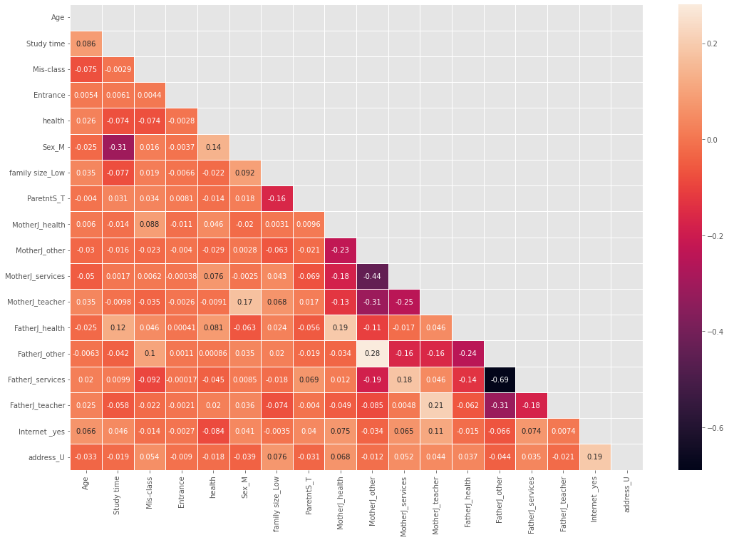
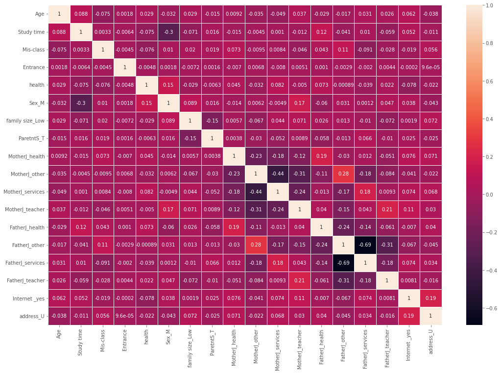
The correlation between different features of the dataset is shown below (see Fig. 5). The correlation score between “Age” and “Study time” is (+ 0.086), which shows that there will be a positive and significant relationship between “Age” and “Study time”. The correlation score between “Age” and “Miss-Class” is (-0.069), which shows that there will be a negative and significant relationship between “Age” and “Miss-Class”. The correlation score between “Age” and “Health” is (+ 0.03), which shows that there will be a positive and significant relationship between “Age” and “Health”. The correlation score between “Age” and “Entrance” is (-0.0035), which shows that there will be a negative and significant relationship between “Age” and “Entrance”. The correlation score between “Age” and “CGPA” is (+ 0.0058), which shows that there will be a positive and significant relationship between “Age” and “CGPA”. The correlation score between “Study time” and “CGPA” is (+ 0.011), which shows that there will be a positive and significant relationship between “Study time” and “CGPA”. The correlation score between “Study time” and “Miss-Class” is (+ 0.002), which shows that there will be a positive and significant relationship between “Study time” and “Miss-Class”. The correlation score between “Study time” and “Health” is (-0.076), which shows that there will be a positive and significant relationship between “Study time” and “Health”. The correlation score between “Study time” and “Entrance” is (+ 0.0011), which shows that there will be a positive and significant relationship between “Study time” and “Entrance”. The correlation score between “Miss-Class” and “Entrance” is (+ 0.00097), which shows that there will be a positive and significant relationship between “Miss-Class” and “Entrance”. The correlation score between “Miss-Class” and “Health” is (-0.072), which shows that there will be a negative and significant relationship between “Miss-Class” and “Health” The correlation score between “Miss-Class” and “CGPA” is (+ 0.0075), which shows that there will be a positive and significant relationship between “Miss-Class” and “CGPA”. The correlation score between “Entrance” and “CGPA” is (+ 0.037), which shows that there will be a positive and significant relationship between “Entrance” and “CGPA”. The correlation score between “Entrance” and “Health” is (-0.0033), which shows that there will be a negative and significant relationship between “Entrance” and “Health”. The correlation score between “Health” and “CGPA” is (+ 0.064), which shows that there will be a positive and significant relationship between “Health” and “CGPA”. Moreover, CGPA has positive relationship with “Age”, “Study time”,” Miss-Class”, “Entrance result ”, and “Health”. “Health” has negative relationship with “Study time”, “Miss-Class”, “Entrance result” but, positive relationship with “CGPA” and “Age”.
Performance Comparison of Developed Models before Smoothing
Performance comparison on five models under Machine learning classier before smoothing are performed and ranked based on the accuracy score. These Machines learning classier were namely: (i.e., SVM, RF, KNN, GBOOST and DECISION TREE,) were applied to predict students’ performance (see Fig. 6).
Performance Comparison of Developed Models after Smoothing
Performance comparison on five models after smoothing under Machine learning classier are performed and ranked based on the accuracy score. These Machines learning classier were namely: (i.e., SVM, RF, KNN, GBOOST and DECISION TREE) were applied to predict students’ performance (see Fig. 7).
Figure 8 Confusion matrix of (a) Random Forest (RF), (b) Gradient Boosting Classifiers Model (GB), (c) Support Vector Machine (SVM) Model (d) K-Nearest Neighbor Classifier (KNN) Model and (e) Decision Tree (DT) Classifier Model
To develop a model An experiment was conducted on a student performance dataset using random forest classifiers. An experiment was conducted on default random forest parameters with a confusion matrix (see Fig. 8(A)). The result from the confusion matrix shows that out of 17,826 instances, 17,622 were correctly classified by the model, and 204 instances were incorrectly classified. Under the Random Forest classifier, out of 3528 samples of students supposed to be warned, 3488 instances were predicted correctly, and 40 samples were incorrectly classified. Under the Random Forest classifier, out of 3514 samples of students supposed to pass, 3404 instances are predicted correctly, and 110 samples are incorrectly classified. Under the Random Forest classifier, out of 3,633 samples of students supposed to be DROPOUT, 3,630 instances are predicted correctly, and 3 samples are only incorrectly classified. Under the Random Forest classifier, out of 3,561 samples of students supposed to be academic dismissal with readmission (ADR), 3539 instances are predicted correctly, and 22 samples are incorrectly classified.
Under the Random Forest classifier, out of 3,590 samples of students supposed to be academic dismissal with readmission (AD), 3561 instances are predicted correctly, and 29 samples are incorrectly classified. Under the Random Forest Classifier Model, training accuracy of 89.5% and testing accuracy of 89% were obtained (see Fig. 8(A)). The results of the random forest classifier revealed that the training accuracy of 89.5% and the testing accuracy of 89% obtained were comparable, thus there is no overfitting in the model. To develop a model, an experiment was conducted on a student performance data set using gradient-boosting classifiers. An experiment was conducted on gradient-boosting default parameters with a confusion matrix (see Fig. 8(B)). The result from the confusion matrix is that out of 17,835 instances, 13798 were correctly classified by the model, and 4037 instances were incorrectly classified. With Gradient Boosting Classifiers, out of 3537 samples of students supposed to be warned, 2455 instances are predicted correctly, and 1082 samples are incorrectly classified. With Gradient Boosting Classifiers, out of 3514 samples of students supposed to pass, 2500 instances are predicted correctly, and 1014 samples are incorrectly classified. With Gradient Boosting Classifiers, out of 3,633 samples of students supposed to be dropped out, 3,558 instances are predicted correctly, and 75 samples are only incorrectly classified. With Gradient Boosting Classifiers, out of 3,561 samples of students supposed to be Academic Dismissal with Readmission (ADR), 2471 instances are predicted correctly, and 1090 samples are incorrectly classified. Gradient Boosting Classifiers: Out of 3,590 samples of students supposed to be Academic Dismissal with Readmission (AD), 2814 instances are predicted correctly, and 776 samples are incorrectly classified. The result of the gradient boosting classifier revealed that the training accuracy of 77.7% and the testing accuracy of 77.3% obtained were comparable, thus there is no overfitting seen in the model. To develop a model, an experiment was conducted on a student performance data set using the SVM classifier model. An experiment was conducted with a confusion matrix (see Fig. 8(C)). The result from the confusion matrix is that out of 17,835 instances, 17,633 were correctly classified by the model, and 202 instances were incorrectly classified. With the SVM Classifier Model, out of 3537 samples of students supposed to be warned, 3480 instances are predicted correctly, and 57 samples are incorrectly classified. With the SVM model, out of 3514 samples of students supposed to pass, 3417 instances are predicted correctly, and 97 samples are incorrectly classified. With the SVM Classifier Model, out of 3,633 samples of students supposed to be dropped out, 3,632 instances are predicted correctly, and 1 sample is only incorrectly classified. With the SVM model, out of 3,561 samples of students supposed to be academic dismissal with readmission (ADR), 3537 instances are predicted correctly, and 24 samples are incorrectly classified. With the SVM Classifier Model, out of 3,590 samples of students supposed to be academic dismissal with readmission (AD), 3567 instances are predicted correctly, and 23 samples are incorrectly classified. With the SVM classifier model, an accuracy of 98.7% was obtained (see Fig. 8(C)). Under the support vector machine classifier model, an accuracy of 98.1% was achieved.
The results of the SVM classifier revealed that the training accuracy of 99.7% and the testing accuracy of 98.1% obtained were comparable. Thus, there is no overfitting in the model. To develop a model, an experiment was conducted on a student performance data set using the KNN classifier model. An experiment was conducted with a confusion matrix (see Fig. 8(D)). The result from the confusion matrix is that out of 17,835 instances, 15,270 were correctly classified by the model, and 2565 instances were incorrectly classified. With the voting classifier, out of 3,537 samples of students supposed to be warned, 3396 instances were predicted correctly, and 141 samples were incorrectly classified. With the KNN classifier, out of 3,514 samples of students supposed to be passing, 1336 instances are predicted correctly, and 2178 samples are incorrectly classified. With the KNN classifier, out of 3,633 samples of students supposed to be dropped out, 3561 instances are predicted correctly, and 72 samples are only incorrectly classified. With the KNN classifier, out of 3,561 samples of students supposed to be academic dismissal with readmission (ADR), 3456 instances are predicted correctly, and 105 samples are incorrectly classified. With the KNN classifier, out of 3,590 samples of students supposed to be academic dismissal with readmission (AD), 3521 instances are predicted correctly, and 69 samples are incorrectly classified. With the KNN classifier model, an accuracy of 85.6% was achieved (see Fig. 8(E)). The results of the KNN classifier revealed that the training accuracy of 86% and the testing accuracy of 85.6% obtained were comparable, thus there is no overfitting seen in the model. To develop a model, an experiment was conducted on the student performance data set using the Decision Tree Classifier Model. An experiment was conducted with a confusion matrix (see Fig. 8(E)). The result from the confusion matrix is that out of 17,835 instances, 17,633 were correctly classified by the model, and 202 instances were incorrectly classified. With the Decision Tree Classifier Model, out of 3537 samples of students supposed to be warned, 3480 instances are predicted correctly, and 57 samples are incorrectly classified. With the Decision Tree Classifier Model, out of 3514 samples of students supposed to pass, 3417 instances are predicted correctly, and 97 samples are incorrectly classified. With the Decision Tree Classifier Model, out of 3,633 samples of students supposed to be DROPOUT, 3,632 instances are predicted correctly, and 1 sample is only incorrectly classified. With the Decision Tree Classifier Model, out of 3,561 samples of students supposed to be Academic Dismissal with Readmission (ADR), 3537 instances are predicted correctly, and 24 samples are incorrectly classified. With the Decision Tree Classifier Model, out of 3,590 samples of students supposed to be academic dismissals with readmission (AD), 3567 instances are predicted correctly, and 23 samples are incorrectly classified. With the decision tree classifier model, an accuracy of 98.7% was obtained, as illustrated in Fig. 7 and Table 4(E).
Table 4 Classification Report of (A) Random Forest(RF),(B) Support Vector Machine Model(SVM),(C) Gradient Boosting(GB) Classifiers Model,(D) Decision Tree(DT) Classifier Model and (E) K-Nearest Neighbor Classifier(KNN) Model
|
(A)
|
(B)
|
(C)
|
|||||||||||||||||||||||||||||||||||||||||||||||||||||||||||||||||||||||||||||||||||||||||||||||||||||||||||||||||||||||||||||||||||||||||||||||||
|
(D)
|
(E)
|
|
|||||||||||||||||||||||||||||||||||||||||||||||||||||||||||||||||||||||||||||||||||||||||||||||||||||||||||||||||||||||||||||||||||||||||||||||||
Hyper Parameter Tuning
Selecting the best hyperparameters could greatly affect the performance of the model [46, 47]. A given algorithm will have several optimisation techniques, each of which has its own drawbacks and pitfalls. In this study, experiments will be conducted on several optimisation methodologies to choose the best hyperparameters. These chosen hyperparameters will be employed in K-Nearest Neighbours, Support Vector Machines, Gradient Boosting, Decision Trees, and Random Forest models).Basically, there are two types of parameters. These are the default parameters of the model and hyperparameters. The learning process will be regulated by the parameters. Different learning rates or weights will be utilised to govern the learning process and uncover hidden knowledge in the data under the same machine learning model. In this study, we employed grid search-based hyperparameter tuning techniques. The reason we select grid search-based hyperparameter tuning over random search-based hyperparameter tuning is because grid search-based hyperparameter tuning techniques go through every possible combination of hyperparameters [48–50]. Thus, it will boost the testing accuracy of the model. In this study, we will employ the grid search-based hyperparameter tuning technique. The reason we select grid search-based hyperparameter tuning over random search-based hyperparameter tuning is because grid search-based hyperparameter tuning techniques go through every possible combination of hyperparameters. It will boost the testing accuracy of the model.
Performance Comparison of Developed Models after Hyper parameter Tuning
Performance comparison on five models after hyper tuning under Machine learning classier are performed and ranked based on the accuracy score. These Machines learning classier were namely: (i.e., SVM, RF, KNN, GBOOST and DECISION TREE) were applied to predict students’ performance (see Fig. 9).
Performance-based comparisons of all models with and without smoothing were discussed. Moreover, the effect of hypertuning on improving the performance of the proposed model was discussed. To determine the best classifier for predicting student performance in the dataset, we examined five machine learning classes, namely: SVM, RF, KNN, GBOOST, and DECISION TREE, which were applied to predict students’ performance. Experiments were conducted before and after smoothing (see Table 5). Before smoothing technique on imbalanced data, Decision Tree surpasses all models in both training and testing accuracy by scoring 99.8% of training accuracy and 97% of testing accuracy. However, it scores the same testing accuracy of 97% with SVM and Random Forest. After the smoothing technique was carried out, imbalanced data were balanced, and Decision Tre scored 99.8% of training accuracy and achieved the highest training accuracy among all models. And the least testing accuracy of 77% was achieved by gradient boosting among all models. After smoothing techniques performed on imbalanced data, the SVM ensemble model outperformed all models with a testing accuracy of 98.8%. An uncomfortable training accuracy of 20% was obtained. The result achieved by SVM shows the existence of underfitting in the model. Therefore, hyperparameter tuning is suggested to address the problem of underfitting seen in the model. Then, the hyper-tuning technique was followed, and the least result was achieved by gradient boosting with a testing accuracy of 47%, and the highest result on test accuracy of 97.3% was achieved by the decision tree (see Table 6) among all models after hyper-tuning techniques were applied. Moreover, the decision tree is a better fitted as training and test accuracy of 97.1% and 97.3% were achieved respectively. Therefore, a decision tree is selected to build the model, and finally, this model is proposed in the study.
| Before Smoothing | After Smoothing | |||
|---|---|---|---|---|
| Models | Training Accuracy | Testing Accuracy | Training Accuracy | Testing Accuracy |
| KNN | 97.2% | 97% | 86.1% | 85.6% |
| Random Forest | 97.2% | 97% | 89.5% | 88.9% |
| Gradient Boost | 97.4% | 96.9% | 77% | 77% |
| Decision Tree | 99.8% | 97% | 99.8% | 97.4 |
| SVC | 97.2% | 97% | 20% | 98.8 |
| Default Models | After Hyper tuning Parameters applied | |||
|---|---|---|---|---|
| Models | Training Accuracy | Testing Accuracy | Training Accuracy | Testing Accuracy |
| KNN | 86.1% | 85.6% | 99.7 | 97.1% |
| Random Forest | 89.5% | 88.9% | 98 | 97.1% |
| Gradient Boost | 89.5% | 97.3% | 47% | 47% |
| Decision Tree | 99.8% | 97.4 | 97.2% | 97.3% |
| SVC | 20% | 98.8 | 97.1% | 96.4% |
Features Importance
Feature selection is the process of selecting essential features that are more uniform, non-redundant, and relevant for a machine learning model [51]. It is recommended to use feature selection because it helps to reduce the size and complexity of the dataset, which in turn requires less time to train a model and requires less computation cost to train a machine learning model. The student academic performance dataset has several features, and all features are not equally affecting the student's academic performance. Besides, all features are not equally important in affecting student academic performance. The purpose of this is to identify the features that have a significant impact on students’ academic performance. After training the prediction model, the decision tree model calculated feature importance by ranking the features. Features such as: entrance result, age, health, study time, father job, mother job, attendance, internet access, parents, sex, family size and address, extra class, another job, guidance, and counselling ranked as follows (see Fig. 9). The same features were also extracted by the second achieved Random Forest classifiers and the first three rank completely the same with the feature extracted by Decision Tree Classifiers. However, the academic performance of students was either lesser or not affected by additional features like extra classes, Another Job, and guidance and counselling. Therefore, they are eliminated and not further considered for the prediction of the model.
Using machine learning (ML) methods, educational data mining (EDM) is used to extract and identify interesting patterns from educational institutions databases [52]. This study aims to develop a machine learning model (ML) based on student statistics to forecast the students' early academic achievement. Several machine learning algorithms (i.e., SVM, RF, KNN, GBOOST, and Decision Tree) were applied to predict students’ performance. The Decision Tree models overtook other models by scoring a promising result of 97.3% and were selected as the proposed model. We applied the parameter tuning technique to obtain the top parameter values that gave us the best results. And then, the performance of the model improved to 97.3%. After parameter tuning was performed, the most important features affecting students’ performance were identified: Entrance result, study time, attendance, Internet, age, gender, father job, mother job, family size, and address were extracted. Our findings suggest that academic factors (entrance result, study time, attendance, and Internet access) and socio-demographic factors (age, gender, father job, mother job, family size, and address) had a greater influence on students' academic success. The academic performance of students was less or not affected by additional features like extra classes, another job, and guidance and counselling. The proposed model is considered an early warning method used by decision-makers to identify students at risk. Once the risks are identified, it is easy to take countermeasures. The proposed model is able to identify problems with students before they get worse. Therefore, a cloud-based student performance prediction model is developed, and a streamlit cloud is proposed to ease use. Student performance prediction models can help educational institutions take timely actions, like arranging appropriate training for students at risk, to increase their success rate. Moreover, this study contributed to the prediction model proposed to classify student status at a finer-grained level, such as ‘pass’, ’warning’, ‘academic dismissal with readmission’, ’academic and ‘dropout’ that haven’t yet been considered in previous work.
The focus of this study is on Bule Hora University students’ academic performance prediction, and only three semesters of data are used. In the future, we intend to include the whole semester of student performance data. Moreover, the study focused on undergraduate students; however, in the future, we will include graduate students. There are also other factors that have to be included in the dataset, like ‘weather condition', 'motivation’, ‘interest on the joined campuses, and ‘interest on the joined department’. In this study, the student entrance result is the only variable used from the pre-university data; however, transcript data during preparatory was not included. Therefore, in the future, we will include transcript information found during preparatory time. The study focuses on the prediction of student performance with five status: ‘warning’, ’pass’, ’academic dismissal’, ‘academic dismissal with readmission’, and ‘dropout’. However, it doesn’t show any kind of recommendation on the action the students must take to improve their performance. In this study, machine learning techniques were utilized to extract hidden knowledge from the student academic performance dataset. In the future, we will train and test the model using deep learning techniques. Moreover, we will develop an application to facilitate instruction for learners by integrating student academic performance prediction models into the mobile application to promote the utilization of modern technology. The stakeholders of the university have to collaboratively engage in working on the factors affecting student academic performance that were identified and prioritized by the model. Special attention with prioritization has to be provided for low achieving students with ‘Warning’, ‘Academic Dismissal with Readmission (ADR)’, ‘Academic Dismissal (AD)’ status. In the future, we will also consider "pass" status at a finer-grained level: Very Great Distinction, Great Distinction, Distinction, and Promoted. This will also encourage students to upgrade their grade and remain competent and productive. However, a CGPA result is not sufficient to qualify a student. Therefore, in the future, the exit exam results of the students will be included.
EDM: Educational Data Mining; HEIs: Higher Educational Institutions; ML: Machine Learning; SVM: Support Vector Machine; DT: Decision Tree; RF: Random Forest; GB: Gradient Boosting; KNN: K-Nearest Neighbor; LMS: Learning management system; ADR: Academic Dismissal with Readmission; AD: Academic Dismissal; SRS: Student Record System; SMOTE: Synthetic Minority Oversampling Technique; MOE: Ministry of Education; BHU: Bule Hora University; CGPA: Cumulative Grade Point Average; MAPE: Mean Absolute Percentage Error; DM: Data Mining
Availability of data and materials
The datasets used and/or analyzed during the current study are available from the corresponding author on reasonable request.
Funding
Not applicable
Authors' contributions
All authors contributed and approved the final manuscript.
Acknowledgements
The authors are thankful to the study participants, data collectors, and supervisors.
Ethics approval and consent to participate
Not applicable.
Consent for publication
Not applicable.
Competing interests
The authors declare no competing interests.
- R. S. Baker, T. Martin, L. M. J. T. W. h. o. c. Rossi, m. assessment: Frameworks, and applications, "Educational data mining and learning analytics," pp. 379-396, 2016.
- C. Romero, S. J. I. T. o. S. Ventura, Man,, and P. C. Cybernetics, "Educational data mining: a review of the state of the art," vol. 40, no. 6, pp. 601-618, 2010.
- P. Kaewsaiha, S. J. E. Chanchalor, and I. Technologies, "Factors affecting the usage of learning management systems in higher education," vol. 26, pp. 2919-2939, 2021.
- C. Romero, S. J. W. i. r. D. m. Ventura, and k. discovery, "Educational data mining and learning analytics: An updated survey," vol. 10, no. 3, p. e1355, 2020.
- C. Romero, S. J. W. I. R. D. m. Ventura, and k. discovery, "Data mining in education," vol. 3, no. 1, pp. 12-27, 2013.
- S. Hussain and M. Q. J. A. o. d. s. Khan, "Student-performulator: Predicting students’ academic performance at secondary and intermediate level using machine learning," vol. 10, no. 3, pp. 637-655, 2023.
- P. Balaji, S. Alelyani, A. Qahmash, and M. J. A. S. Mohana, "Contributions of machine learning models towards student academic performance prediction: a systematic review," vol. 11, no. 21, p. 10007, 2021.
- K. Fahd, S. Venkatraman, S. J. Miah, K. J. E. Ahmed, and I. Technologies, "Application of machine learning in higher education to assess student academic performance, at-risk, and attrition: A meta-analysis of literature," pp. 1-33, 2022.
- M. J. S. L. E. Yağcı, "Educational data mining: prediction of students' academic performance using machine learning algorithms," vol. 9, no. 1, p. 11, 2022.
- P. Goldberg et al., "Attentive or not? Toward a machine learning approach to assessing students’ visible engagement in classroom instruction," vol. 33, pp. 27-49, 2021.
- S. B. J. A. I. R. Kotsiantis, "Use of machine learning techniques for educational proposes: a decision support system for forecasting students’ grades," vol. 37, pp. 331-344, 2012.
- M. Hussain, W. Zhu, W. Zhang, S. M. R. Abidi, and S. J. A. I. R. Ali, "Using machine learning to predict student difficulties from learning session data," vol. 52, pp. 381-407, 2019.
- S. B. Kotsiantis, C. Pierrakeas, and P. E. Pintelas, "Preventing student dropout in distance learning using machine learning techniques," in Knowledge-Based Intelligent Information and Engineering Systems: 7th International Conference, KES 2003, Oxford, UK, September 2003. Proceedings, Part II 7, 2003, pp. 267-274: Springer.
- J. E. Beck and B. P. Woolf, "High-level student modeling with machine learning," in International Conference on Intelligent Tutoring Systems, 2000, pp. 584-593: Springer.
- S.-C. Tsai, C.-H. Chen, Y.-T. Shiao, J.-S. Ciou, and T.-N. J. I. J. o. E. T. i. H. E. Wu, "Precision education with statistical learning and deep learning: a case study in Taiwan," vol. 17, pp. 1-13, 2020.
- I. M. K. Ho, K. Y. Cheong, and A. J. P. o. Weldon, "Predicting student satisfaction of emergency remote learning in higher education during COVID-19 using machine learning techniques," vol. 16, no. 4, p. e0249423, 2021.
- P. C. McKee, C. J. Budnick, K. S. Walters, and I. J. P. o. Antonios, "College student Fear of Missing Out (FoMO) and maladaptive behavior: Traditional statistical modeling and predictive analysis using machine learning," vol. 17, no. 10, p. e0274698, 2022.
- O. Weller, L. Sagers, C. Hanson, M. Barnes, Q. Snell, and E. S. J. P. o. Tass, "Predicting suicidal thoughts and behavior among adolescents using the risk and protective factor framework: A large-scale machine learning approach," vol. 16, no. 11, p. e0258535, 2021.
- Y. Zhao, Y. Ding, H. Chekired, and Y. J. P. o. Wu, "Student adaptation to college and coping in relation to adjustment during COVID-19: A machine learning approach," vol. 17, no. 12, p. e0279711, 2022.
- Z. Papamitsiou, A. A. J. J. o. E. T. Economides, and Society, "Learning analytics and educational data mining in practice: A systematic literature review of empirical evidence," vol. 17, no. 4, pp. 49-64, 2014.
- F. Marbouti, H. A. Diefes-Dux, K. J. C. Madhavan, and Education, "Models for early prediction of at-risk students in a course using standards-based grading," vol. 103, pp. 1-15, 2016.
- J. L. Rastrollo-Guerrero, J. A. Gómez-Pulido, and A. J. A. s. Durán-Domínguez, "Analyzing and predicting students’ performance by means of machine learning: A review," vol. 10, no. 3, p. 1042, 2020.
- K. A. Kaufman and R. S. Michalski, "Learning from inconsistent and noisy data: the AQ18 approach," in International Symposium on Methodologies for Intelligent Systems, 1999, pp. 411-419: Springer.
- A. Fatima, N. Nazir, and M. G. J. I. J. I. T. C. S. Khan, "Data cleaning in data warehouse: A survey of data pre-processing techniques and tools," vol. 9, no. 3, pp. 50-61, 2017.
- A. Manca, S. J. A. h. e. Palmer, and h. policy, "Handling missing data in patient-level cost-effectiveness analysis alongside randomised clinical trials," vol. 4, pp. 65-75, 2005.
- I. Triguero et al., "Transforming big data into smart data: An insight on the use of the k‐nearest neighbors algorithm to obtain quality data," vol. 9, no. 2, p. e1289, 2019.
- P. Hajibabaee, F. Pourkamali-Anaraki, and M. J. E. S. Hariri-Ardebili, "Dimensionality reduction techniques in structural and earthquake engineering," vol. 278, p. 115485, 2023.
- F. E. Harrell Jr, K. L. Lee, and D. B. J. S. i. m. Mark, "Multivariable prognostic models: issues in developing models, evaluating assumptions and adequacy, and measuring and reducing errors," vol. 15, no. 4, pp. 361-387, 1996.
- L. J. T. D. S. Li, "Principal component analysis for dimensionality reduction," 2019.
- C. Patel et al., "Matching patient records to clinical trials using ontologies," in The Semantic Web: 6th International Semantic Web Conference, 2nd Asian Semantic Web Conference, ISWC 2007+ ASWC 2007, Busan, Korea, November 11-15, 2007. Proceedings, 2007, pp. 816-829: Springer.
- A. Shehadeh, O. Alshboul, R. E. Al Mamlook, and O. J. A. i. C. Hamedat, "Machine learning models for predicting the residual value of heavy construction equipment: An evaluation of modified decision tree, LightGBM, and XGBoost regression," vol. 129, p. 103827, 2021.
- M. M. J. J. o. A. R. i. N. Arat and A. Sciences, "Learning From High-Cardinality Categorical Features in Deep Neural Networks," vol. 8, no. 2, pp. 222-236, 2022.
- A. Zheng and A. Casari, Feature engineering for machine learning: principles and techniques for data scientists. " O'Reilly Media, Inc.", 2018.
- N. K. Visalakshi and J. Suguna, "K-means clustering using Max-min distance measure," in NAFIPS 2009-2009 Annual Meeting of the North American Fuzzy Information Processing Society, 2009, pp. 1-6: IEEE.
- S. M. Fati, A. Muneer, N. A. Akbar, and S. M. J. S. Taib, "A continuous cuffless blood pressure estimation using tree-based pipeline optimization tool," vol. 13, no. 4, p. 686, 2021.
- V. G. Raju, K. P. Lakshmi, V. M. Jain, A. Kalidindi, and V. Padma, "Study the influence of normalization/transformation process on the accuracy of supervised classification," in 2020 Third International Conference on Smart Systems and Inventive Technology (ICSSIT), 2020, pp. 729-735: IEEE.
- D. U. Ozsahin, M. T. Mustapha, A. S. Mubarak, Z. S. Ameen, and B. Uzun, "Impact of feature scaling on machine learning models for the diagnosis of diabetes," in 2022 International Conference on Artificial Intelligence in Everything (AIE), 2022, pp. 87-94: IEEE.
- D. Calvanese, G. De Giacomo, M. Lenzerini, D. Nardi, and R. J. I. J. o. C. I. S. Rosati, "Data integration in data warehousing," vol. 10, no. 03, pp. 237-271, 2001.
- A. Gelman, G. J. J. o. B. Imbens, and E. Statistics, "Why high-order polynomials should not be used in regression discontinuity designs," vol. 37, no. 3, pp. 447-456, 2019.
- S. Park and H. J. C. Park, "Combined oversampling and undersampling method based on slow-start algorithm for imbalanced network traffic," vol. 103, no. 3, pp. 401-424, 2021.
- L. Van der Schraelen, K. Stouthuysen, S. V. Broucke, and T. J. I. S. Verdonck, "Regularization oversampling for classification tasks: To exploit what you do not know," vol. 635, pp. 169-194, 2023.
- P. K. Jadwal, S. Jain, S. Pathak, and B. J. M. T. Agarwal, "Improved resampling algorithm through a modified oversampling approach based on spectral clustering and SMOTE," vol. 28, no. 12, pp. 2669-2677, 2022.
- S. Shukla, A. Maheshwari, and P. Johri, "Comparative analysis of ml algorithms & stream lit web application," in 2021 3rd International Conference on Advances in Computing, Communication Control and Networking (ICAC3N), 2021, pp. 175-180: IEEE.
- T.-T. Wong, P.-Y. J. I. T. o. K. Yeh, and D. Engineering, "Reliable accuracy estimates from k-fold cross validation," vol. 32, no. 8, pp. 1586-1594, 2019.
- M. Al Helal, M. S. Haydar, and S. A. M. Mostafa, "Algorithms efficiency measurement on imbalanced data using geometric mean and cross validation," in 2016 international workshop on computational intelligence (IWCI), 2016, pp. 110-114: IEEE.
- H. Huang, R. Jia, X. Shi, J. Liang, and J. J. A. I. Dang, "Feature selection and hyper parameters optimization for short-term wind power forecast," pp. 1-19, 2021.
- P. Probst, M. N. Wright, A. L. J. W. I. R. d. m. Boulesteix, and k. discovery, "Hyperparameters and tuning strategies for random forest," vol. 9, no. 3, p. e1301, 2019.
- X. Zhang, X. Chen, L. Yao, C. Ge, and M. Dong, "Deep neural network hyperparameter optimization with orthogonal array tuning," in Neural Information Processing: 26th International Conference, ICONIP 2019, Sydney, NSW, Australia, December 12–15, 2019, Proceedings, Part IV 26, 2019, pp. 287-295: Springer.
- J. Bergstra and Y. J. J. o. m. l. r. Bengio, "Random search for hyper-parameter optimization," vol. 13, no. 2, 2012.
- H. Alibrahim and S. A. Ludwig, "Hyperparameter optimization: Comparing genetic algorithm against grid search and bayesian optimization," in 2021 IEEE Congress on Evolutionary Computation (CEC), 2021, pp. 1551-1559: IEEE.
- N. Hoque, M. Singh, D. K. J. C. Bhattacharyya, and I. Systems, "EFS-MI: an ensemble feature selection method for classification: An ensemble feature selection method," vol. 4, pp. 105-118, 2018.
- D. A. Shafiq, M. Marjani, R. A. A. Habeeb, and D. J. I. A. Asirvatham, "Student retention using educational data mining and predictive analytics: a systematic literature review," 2022.
No competing interests reported.