Site description
The study was conducted in the SNNPR, in southwestern Ethiopia (Fig. 1a). The area has a variable topography with an altitude ranging from 340 to 3433 m (Fig. 1b). The south and west of the area comprise flat lowlands, whereas the north and east are mountainous. P. pedifer occurs in mountainous areas and the model village for research on CL transmission, Ochollo, is situated near Arba Minch, in Gamo zone. Therefore, we selected Gamo zone, three additional surrounding administrative zones, including Gofa, Wolaita and Dawuro, and Dherashe area for sample collection (Fig. 1c). Together, the area covers approximately 22,000 km2 and is inhabited by 4.7 million people.
The study area consists of mountains and valleys with an altitude ranging between 550 and 3,390 m. Due to its topography, it has a temperate climate, with an average yearly temperature ranging from 9.3 °C to 25.5 °C and rainfall varying between 630 mm and 2,280 mm respectively in the low- and highlands [31]. Because the study area covers a wide topographical range, the seasons vary from place to place, but generally the dry season lasts from October to April and the wet season from May to September. In recent years, the area has been subjected to ecological modifications related to human activities, like urbanization, agriculture and deforestation.
Occurrence data
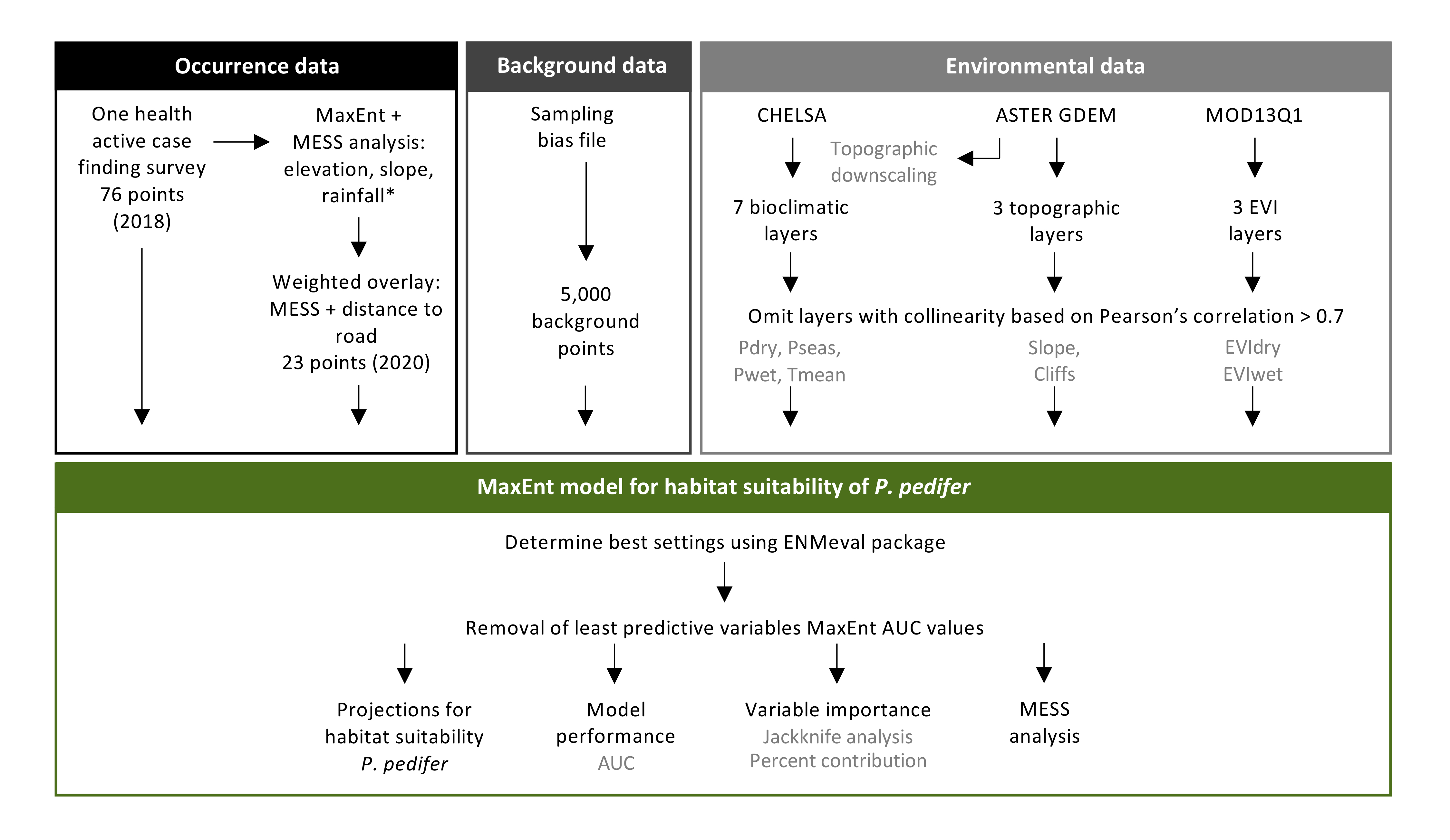
Occurrence points of P. pedifer were collected during two consecutive entomological surveys (Fig. 2 black frame, Fig. 3).
First, 76 presence points were assembled during an active case finding survey carried out from May to July 2018. The survey was performed under guidance of a neglected tropical diseases (NTD) focal person and health extension workers, and by questioning community members about the presence of CL patients supported by pictures of lesions and hyraxes. When a suspected CL case was found, a CDC miniature light trap (John W. Hock Company, Gainesville, Florida, USA) was set in the late afternoon inside the patient’s dwelling or in a nearby cave or rocky area where hyraxes were present. Sand flies were collected the next morning, mounted in CMCP-10 high viscosity mountant (Polysciences Europe, Herschberg, Germany) and the species was determined according to relevant morphological keys [32–34].
Second, an elementary Maximum Entropy (MaxEnt) model was made using the P. pedifer presence points collected during the active case finding survey in 2018 and environmental layers that were found to predict the presence of CL in Ethiopia in a study of Seid and colleagues (2014): altitude, slope and rainfall [17]. A multivariate environmental similarity surface (MESS) analysis was integrated, measuring the extent of the projected data, which was not within the range with the training variables (thus causing model extrapolation). We intended to keep the extent of extrapolation low as it informs on the credibility of the model output. Therefore, a new sampling approach was designed based a weighted overlay of the MESS analysis (70%) and the distance to the road (30%), in order to reduce the degree of extrapolation by additional sampling in accessible places. This entomological survey was carried out in the dry season (January and February 2020), when sampling sites were better accessible and a higher sand fly abundance was expected [16]. During this survey, we searched for suspected CL cases for nearby sand fly trapping. If CL cases were absent, traps were placed in other potential sand fly breeding or resting sites, because the area could still be at risk for an outbreak if the vector would be present. Collected specimens were processed as described above, leading to 23 additional P. pedifer presence points.
Sampling bias file
Most of the sampling effort was performed within a certain distance to the roads and towns (approximately 10 km), which was necessary to ensure access to the sampling areas, particularly at rainy days. Moreover case finding and sand fly trapping were never attempted at altitudes under 1,400 mThis is because neither P. pedifer nor CL have been observed at altitudes under 1,700 m. Additionally, we applied a buffer of 300 m in altitude to avoid missing sites where P. pedifer could be present on one hand and prevent putting too much effort in sites where the vector cannot be found on the other hand.
In order to diminish spatial autocorrelation of the sampled presence points without reducing the predictive power of the model, a sampling bias file was designed to match the sampling effort and avoid overfitting of the model (Fig. 2 dark grey frame, Fig. 3) [35]. Therefore, a weighted overlay was performed with increasing weights for proximity (< 2.5 km, 2.5 - 5 km, 5 km - 10 km, > 10 km) to a town and road (50/50%). All areas under 1,400 m were given the lowest weight and the final raster file was used for selection of background points with an increased probability in areas with a high sampling effort (explained below).
Environmental data
Collection of environmental data
A wide range of environmental layers was acquired as candidate explanatory variables for the model (Fig. 2 light grey frame). Specifics and sources of the variables and the range in our study site are demonstrated in Table 1. All manipulations of the variable layers were carried out in ArcGIS version 10.4.1.
Table 1 Environmental layers acquired as candidate explanatory variables to predict the habitat suitability of Phlebotomus pedifer. CHELSA layers at 30 arcseconds were downscaled and USGS Slope and Cliffs layers were resampled, all to a 250 m spatial resolution. Abbreviations: CHELSA, Climatologies at high resolution for the earth’s land surface areas; USGS: United States Geological Survey.
|
Name
|
Explanation
|
Source
|
Original spatial resolution
|
Data range study area
|
|
Tmean
|
Annual Mean Temperature (Bio1)
|
CHELSA
|
30 arcsec
|
8 – 34 °C
|
|
Tmax
|
Max Temperature of the Warmest Month (Bio5)
|
CHELSA
|
30 arcsec
|
14 – 45 °C
|
|
Tmin
|
Min Temperature of the Coldest Month (Bio6)
|
CHELSA
|
30 arcsec
|
2 – 31 °C
|
|
PrecMean
|
Annual Precipitation (Bio12)
|
CHELSA
|
30 arcsec
|
526 – 3216 mm
|
|
PrecWet
|
Precipitation of the Wettest Month (Bio13)
|
CHELSA
|
30 arcsec
|
90 – 369 mm
|
|
PrecDry
|
Precipitation of the Driest Month (Bio14)
|
CHELSA
|
30 arcsec
|
5 – 68 mm
|
|
PrecSeas
|
Precipitation Seasonality (Bio15)
|
CHELSA
|
30 arcsec
|
21 – 94 %
|
|
Slope
|
Hill slope calculated from elevation DEM
|
USGS
|
30 m
|
0 – 77 %
|
|
Cliffs
|
Ordinal categorical value for number of slopes exceeding 20% and 40% per pixel
|
USGS
|
30 m
|
1 – 9
|
|
EVImean
|
Average EVI from January 2017 until December 2019 – MOD13Q1
|
USGS
|
250 m
|
-0.13 – 0.59
|
|
EVIdry
|
Average EVI for the dry season (January to March) – MOD13Q1
|
USGS
|
250 m
|
-0.99 – 0.60
|
|
EVIwet
|
Average EVI for the wet season (July to September) – MOD13Q1
|
USGS
|
250 m
|
-0.16 – 0.70
|
Because temperature and precipitation are relevant drivers for the distribution of P. pedifer, bioclimatic variables were derived from ‘Climatologies at high resolution for the earth’s land surface areas’ (CHELSA, https://chelsa-climate.org/bioclim/) with a spatial resolution of 30 arcsec (~1 km) [16,31]. A subset of seven out of 19 available bioclimatic variables were considered ecologically relevant to the species and selected, in particular annual averages and extrema (minimum and maximum) for both temperature and precipitation and a variable describing the annual rainfall variation as a measure for seasonality [36].
The vector is breeding in caves on cliff walls, where hyraxes are living. Therefore, an ASTER digital elevation model (DEM) with 30 m spatial resolution was acquired from U.S. Geological Survey (USGS, earth explorer, https://earthexplorer.usgs.gov/), of which the slope (percentage) was computed. To avoid losing the information about cliffs while resampling to a resolution of 250 m, an additional ordinal categorical layer was created using a weighted overlay analysis, indicating number of slopes between 20% - 40% (25% weight), and > 40% (75% weight) per 250 m pixel.
Sand flies require vegetation through which they can move, forage and reproduce [37]. Hence, vegetation layers were included as potential predictors from USGS. The Moderate Resolution Imaging Spectroradiometer (MODIS) enhanced vegetation index (EVI) quantifies the vegetation density. The MOD13Q1 product (https://earthexplorer.usgs.gov/) is produced on a 16 days interval base and corrects for particular atmospheric conditions and canopy background noise. Indices were derived for the annual and seasonal averages over the past three years (2017-2019) with 250 m spatial resolution.
All environmental layers, the occurrence points and bias file were projected in the same spatial reference system, World Geodetic System 84 (WGS84 EPSG:4326).
Topographic downscaling of climate layers
The bioclimatic layers were downscaled on the basis of topographic variables to produce topoclimate (local climate at a particular topography) at high resolution as functionally relevant predictor variables [38]. We opted for a resolution of 250 m because it formed an appropriate balance between a feasible spatial resolution to guide implementation of vector control measures and the computational capacity required for the downscaling process. Downscaling followed a Geographically Weighted Regression (GWR) approach [39] outlined by Lenoir et al. [40] and was based on elevation, slope, northness, eastness, distance from the ocean, and potential solar radiation. These predictor variables have shown good results for predicting temperature and precipitation data in previous studies [40–46].
Data were prepared for downscaling in R version 3.5.2 [47] using the raster package [48]. The area was subdivided into 16 sections to make the computation time for downscaling feasible for the size of our study site. Topographic variables were derived from the ASTER DEM at 250 m resolutionDistance from the ocean was downloaded from http://www.soest.hawaii.edu/pwessel/gshhg/ at 1 arcmin resolution [49]. The potential incoming solar radiation was calculated for each grid cell of the DEM for the spring equinox (March 21st) with a six-hour resolution using the SAGA GIS 6.3.0 tool Potential Incoming Solar Radiation [50]. The downscaling was performed on resources provided by the NTNU IDUN/EPIC computing cluster using R version 3.6.0 and the spgwr package [51]. The 16 sections were mosaicked together and checked for correspondence to CHELSA values. Single outliers due to small bandwidth of the GWR were removed and missing data were interpolated using the Close Gaps tool of SAGA.
Variable preparation
Overall, 12 environmental layers were considered to potentially predict the habitat suitability of P. pedifer (Table 1). All layers were resampled to match a 250 m spatial resolution. For aggregation of the slope variable, the maximum values were retained to prevent the loss of information on slope steepness, while for all other layers, average values were calculated.
Apart from ecological relevance, multi-collinearity among candidate predictor variables was assessed with a Pearson’s correlation (Fig. 2 light grey frame, Additional file 1: Fig. S1). If the absolute coefficient exceeded 0.7, one of the pair variables was omitted for inclusion in the model. This resulted in eight remaining candidate predictor variables: Tmean, Pmean, Pdry, Pseas, Slope, Cliffs, EVIdry and EVIwet.
MaxEnt model implementation
A model predicting the habitat suitability of P. pedifer was developed by a MaxEnt model using the dismo package in R version 3.3.1 [52].
The optimal settings for the MaxEnt model were determined using the ENMeval R package, in which the random 10-fold cross-validation data partitioning method was used (Fig. 2 green frame) [53,54]. The function compares all possible model setting combinations and calculates the Akaike information criterion (AIC) value for each combination. The lowest AIC value was found for a model with a regularization multiplier of 0.5, including linear and quadratic features and a combination of these classes. Hence, these settings were used to fit the model, which was run using a 10-fold cross-validation method, with 75% of the presences used for training and 25% for testing. Additionally, 5,000 background points were assigned based on the bias file (Fig. 3).
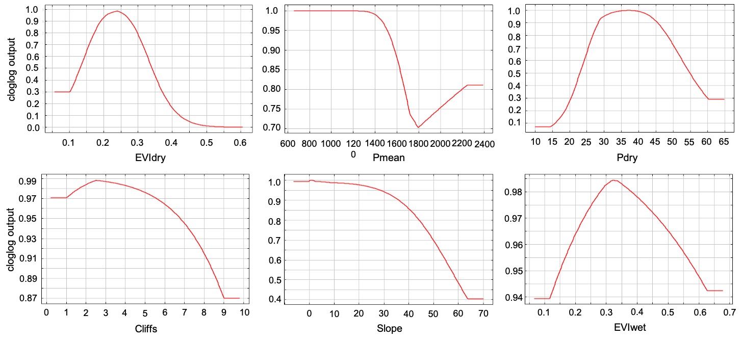
A second round of variable selection was carried out by an iterative removal of the least predictive variables by the area under the curve (AUC) values of the receiver operator characteristic (ROC) of the MaxEnt model to maximize the model performance and minimize overfitting. Yet, all variables contributed considerably to a better model AUC, so the final model consisted of the following eight variables: Tmean, Pmean, Pdry, Pseas, Slope, Cliffs, EVIdry, EVIwet.
In order to assess the robustness of the final model, it was run 200 times, including new random background points in each run. Model accuracy was evaluated by calculating the average training and testing AUC values over 200 runs.
A MESS analysis was performed to indicate areas where model projections were extrapolated (Fig. 2 green frame).The relative importance of the variables to predict the habitat suitability of P. pedifer was assessed using the jackknife estimates and percent contributions.