Overview
The proposed method can be used to calculate the necessary sample size to reach a required statistical power level (here: 0.8, 80%) for a range of relevant metrics of personal light exposure. The effect size under evaluation is taken from a historical dataset where participants are compared between summer and winter season. The method uses bootstrapping [26] at its core, i.e. sample re-use techniques, and importantly takes higher level (inter-individual) and lower level (intra-individual) variance into account. All metrics use melanopic equivalent daylight (D65) illuminance (mel EDI) as their basis for calculation, defined by the CIE S 026 standard [25].
Dataset
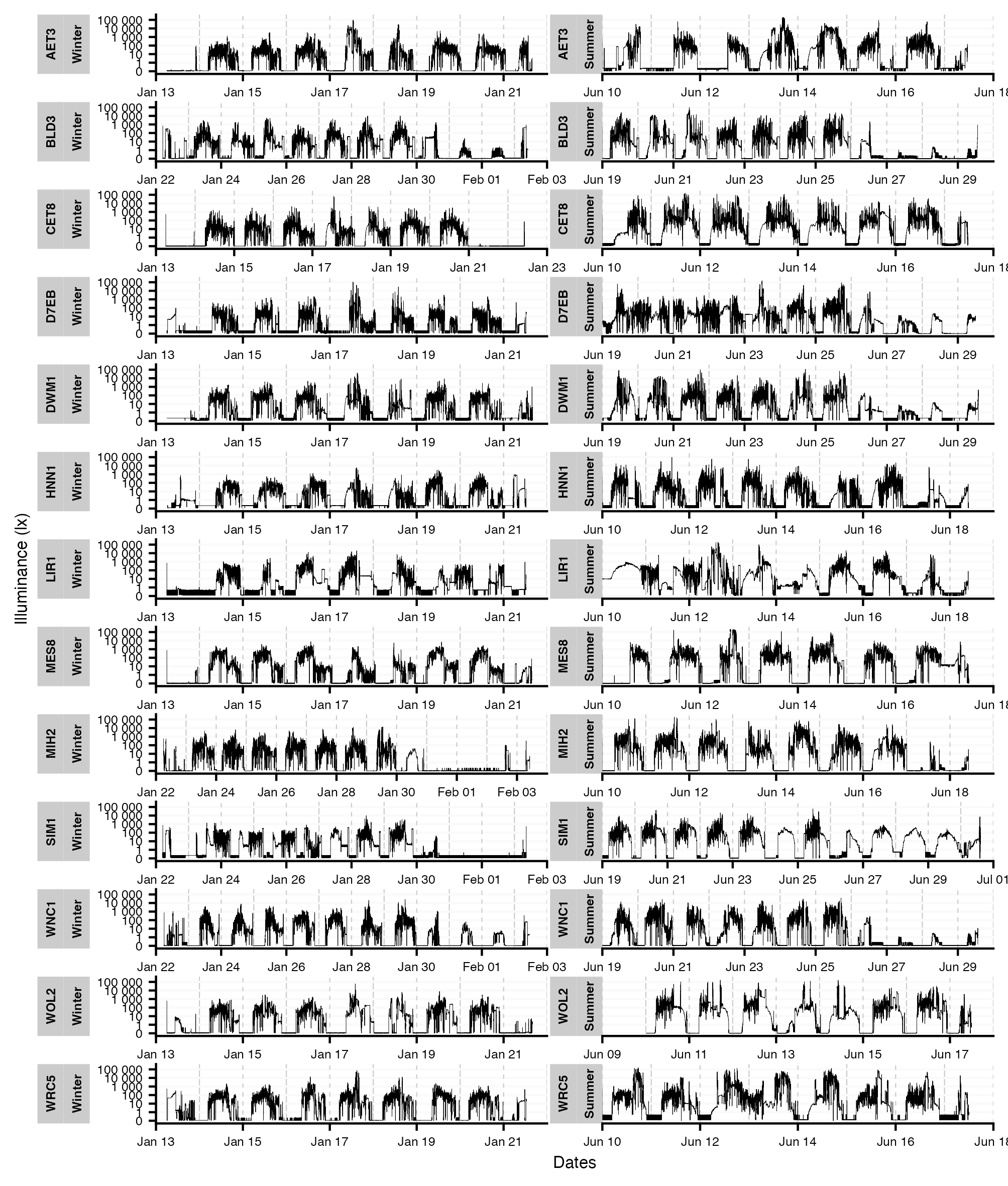
The data used is part of a historical dataset that was collected for a study on evaluating personal light exposure of shift workers in two geographical locations (London and Dortmund) [1]. Light exposure was recorded using the Actiwatch Spectrum device (Philips, Amsterdam) attached on the outer layer of clothing at chest level. The data relate to the Dortmund geolocation branch of that study, and were collected in a field experiment, where participants recorded personal light exposure continuously for a working week with different shift work settings in Winter (Jan/Feb), Spring (Apr, not part of the dataset), and Summer (Jun) 2015. For a more comprehensive description of the study and participants, we refer to the original publication by Price, et al. [1]. The data used in the present analysis are published under a Creative Commons license (CC-BY) on Zenodo (Link to be added after archiving the Github repository https://github.com/tscnlab/ZaunerEtAl_BMCMedResMethodol_2024/).
Software
We used the R software [27], Version 4.2.3 for all analysis. Data pre-processing and visualizations were done with the LightLogR package [28], which is specifically designed to aid in analysis of wearable light logger data. The statistical analysis is based on a linear mixed-effect model, performed with the lme4 package [29], p values are calculated with the lmerTest package [30]. All scripts and results are part of Supplemental Information S1 as an HTML Quarto document [31], including the necessary source code for replication. Reproducibility will be ensured through CODECHECK [32] prior to publication of the peer-reviewed publication.
Data pre-processing
The goal of data pre-processing is to load and clean the datasets, which are export files from the measurement device. Further, values of melanopic EDI are calculated from the sensor data, as well as metrics based on those melanopic EDI. From the potential pool of participants, 13 participants were pre-selected for the analysis at hand, based on the following criteria:
-
At least two days of data, during which the participant worked in the early-day shift (i.e., no night or late shifts), during both the January and June data collection periods.
An early-day shift (day shift from here on out) is defined as working from 06:00 in the morning until 14:00 in the afternoon local time. See Fig. 1 for an overview. Only workdays were selected for analysis.
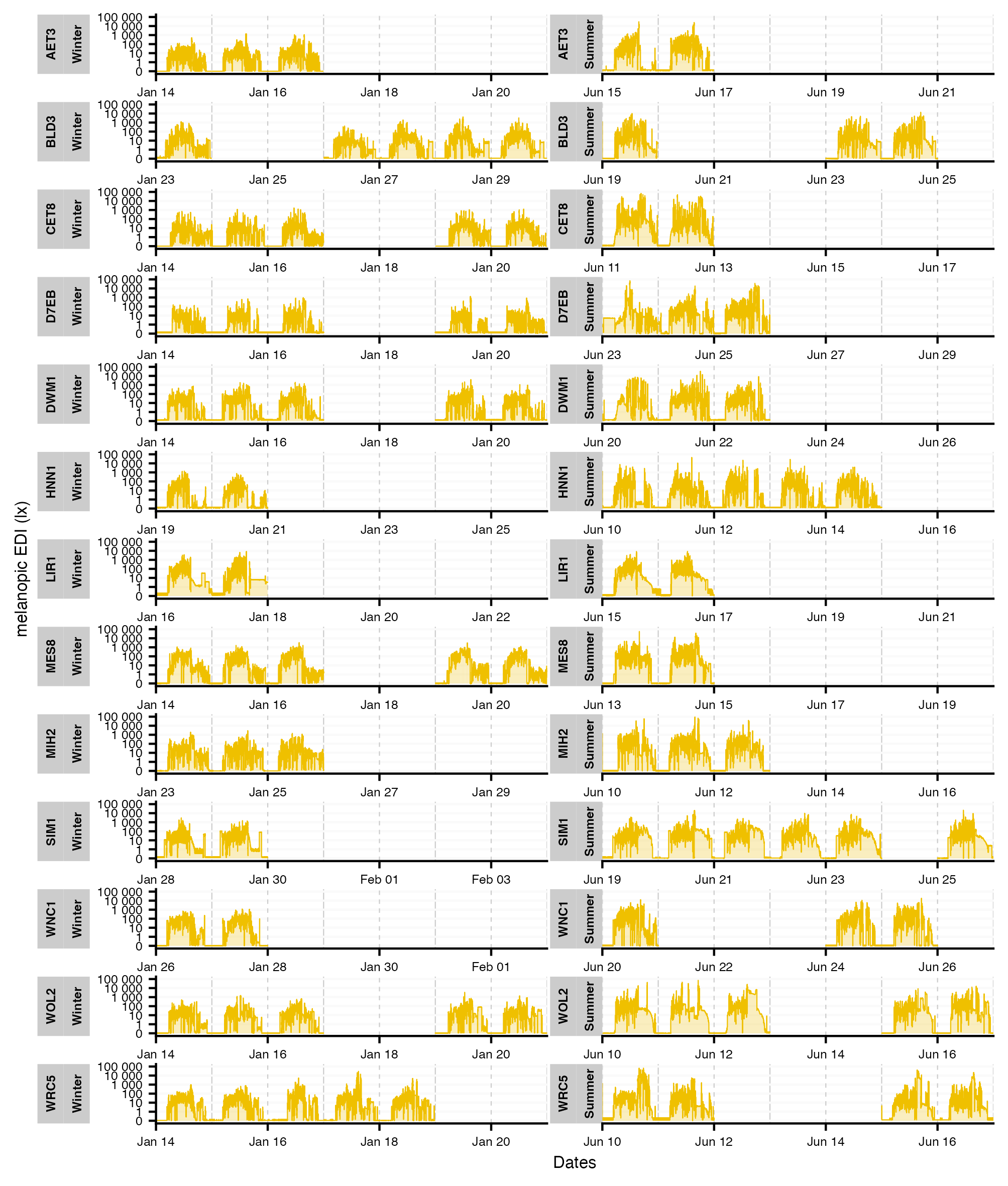
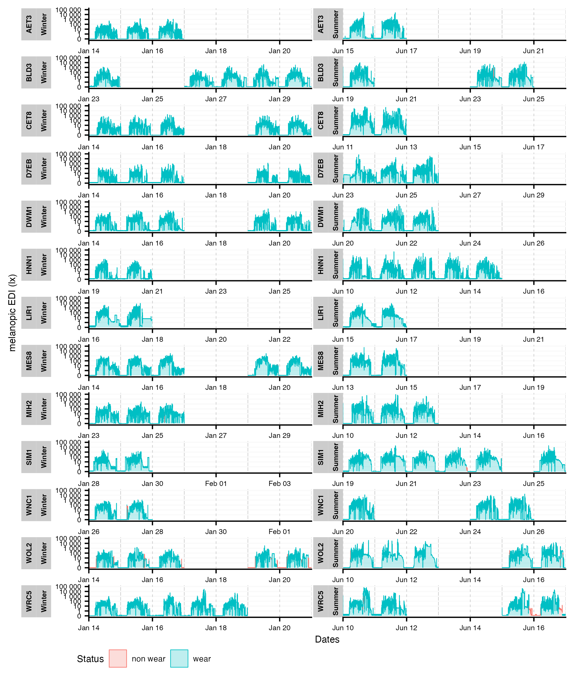
Furthermore, each participant-day needs to have a minimum of 80% valid, non-missing data, or that day will be removed from analysis. Non-missing data are evaluated by a regular sequence of measurement intervals (epochs) that are dominant to the data. Valid data are evaluated by a column of the dataset that indicates whether the device was worn or not. If less than two days per season remain, this participant is removed from analysis. Four days were removed from analysis due to the threshold criterion (see Fig. 2), leaving the total number of participants at 13 and the number of participant-days at 88 (46 in winter, 42 in summer, see Table 1).
Table 1
Summary of remaining and invalid days included in the analysis
|
Characteristic
|
Valid days, n = 881 (96%)
|
Invalid days, n = 41 (4%)
|
|
Season
|
|
|
|
Winter
|
46 (52%)
|
3 (75%)
|
|
Summer
|
42 (48%)
|
1 (25%)
|
|
Invalid/Non-Wear Time
|
0% – 15%
|
24% − 34%
|
|
1n (%); Range
|
The Actiwatch Spectrum device has three sensors that record light exposure in the red, green (G) and blue (B) regions of the visible spectrum, as well as illuminance. In the study of Price, et al. [1] the sensitivities of the G- and B-sensor were linearly combined to give a spectral match to the melanopic action spectrum. Devices were calibrated, and mel EDI was calculated according to:
$${E}_{v, mel}^{D65}=\frac{4.3\left(G+B\right) mW{m}^{-2}}{1.3262 mW{lm}^{-1}}$$
1
Where G and B are the green and blue sensor outputs, respectively. Lastly, for each participant-day, a range of typical wearable light logger related metrics were calculated [17]. These are the basis for the bootstrapping procedure and power analysis. Table 2 shows an overview of used metrics.
Table 2
Overview of calculated metrics, their units, and parametrization
|
Variable name
|
Unit
|
Parameters
|
|
Geometric mean & standard deviation (GM, GSD)
|
lx
|
log base = 10
|
|
Luminous exposure (LE)
|
lx·h
|
-
|
|
Time above threshold (TAT)
|
h
|
thresholds: 250 lx; 1000 lx
|
|
Mean timing of light (MTL)
|
hh:mm
|
above 250 lx, below 10 lx
|
|
Intradaily variability (IV)
|
-
|
-
|
|
Conditional mean & midpoint (M10, L5)
|
lx, hh:mm
|
brightest 10 hours, darkest 5 hours
|
Bootstrapping
The bootstrapping procedure aims to derive at many samples \(\varvec{m}\) for each of a range of sample sizes \(\varvec{n}\) by sampling the dataset with replacement, where \(\varvec{n}\) is the number of participants. Importantly, this procedure takes the intraindividual variance (day-to-day variance of metrics per participant) into account, which differs from traditional bootstrapping procedures, where either no grouping occurs or only the lower level is sampled (i.e., grouping by participant and re-sampling within a participant) [26]:
-
First, the higher order (participants) is sampled with replacement until \(n\) is reached
-
Second, the lower order (daily metrics within participants and between seasons) is resampled with replacement.
The benefit of bootstrapping is the generation of value-pair distributions (winter & summer) based on real variances as captured by the dataset for each metric and depending on \(\varvec{n}\). The range of sample sizes \(\varvec{n}\) in our analysis is 3 to 50 and \(\varvec{m}\) is 1000.
Power analysis
The power analysis aims to detect the minimum sample size, where a threshold criterion of 0.8 power is reached for each metric. Power is calculated as the fraction of significant results compared to all statistical tests at each respective sample size as produced by the bootstrapping procedure. The analyzed model uses the equation (mathematical and Wilkinson notation, respectively)
$${E(\text{Metric}}_{i}\text{) =}{\alpha }_{i}\text{+}{\beta }_{i}* {\text{Season}}_{\text{Winter}}+{b}_{p,i}, {\text{M}\text{e}\text{t}\text{r}\text{i}\text{c}}_{i} \sim 1+\text{S}\text{e}\text{a}\text{s}\text{o}\text{n}+\left(1\right|\text{Participant})$$
2
where\({\text{Metric}}_{i} \sim \left({\mu }_{i}, {{\sigma }^{2}}_{i}\right),{b}_{p,i} \sim N\left(0, {\sigma }_{b,i}^{2}\right)\)
Intercept \({\varvec{\alpha }}_{\varvec{i}}\) and slope \({\varvec{\beta }}_{\varvec{i}}\) are the fixed effects of the model described in Eq. 2. The intercept \({\varvec{\alpha }}_{\varvec{i}}\) indicates the expected value of a respective metric \({\varvec{E}(\text{Metric}}_{\varvec{i}}\text{)}\text{ }\)when all other terms in the equation are zero. The slope, or beta coefficient, \({\varvec{\beta }}_{\varvec{i}}\) represent the change in the expected value of a metric when the season is winter, compared to summer. As random effects we included random intercepts \({\varvec{b}}_{\varvec{p},\varvec{i}}\) by participant \(\varvec{p}\). Random intercepts \({\varvec{b}}_{\varvec{p},\varvec{i}}\) show how much individuals deviate from the average value of a metric (\({\varvec{\alpha }}_{\varvec{i}}\)) with a Gaussian distribution of mean 0 and a variance of \({\varvec{\sigma }}_{\varvec{b},\varvec{i}}^{2}\). For computational stability across the multitude of tests we did not include random slopes. Each metric has a Gaussian distribution, with variance \({{\varvec{\sigma }}^{2}}_{\varvec{i}}\) around its mean \({\varvec{\mu }}_{\varvec{i}}\). The significance level for the fixed effect of Season is set at 0.05.