4.1 Contrast in biological seasonality between zones
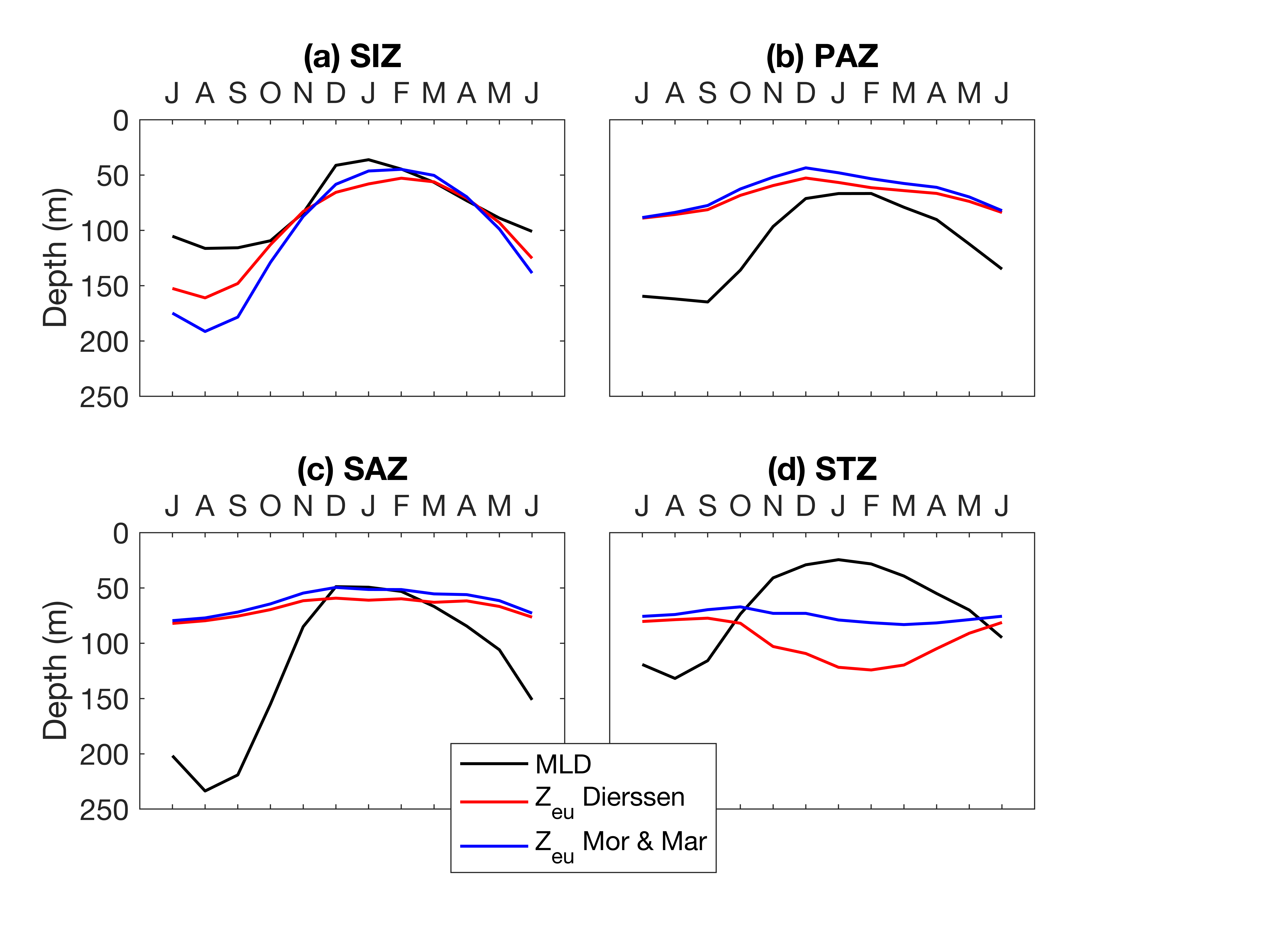
The time series highlights the seasonality in integrated POC production. The timing and magnitude increase southward, except for the SIZ which shows the lowest POC production in surface waters (Fig. 3). In the SIZ, the phytoplankton bloom is strongly influenced by the sea-ice seasonal cycle (Stammerjohn et al., 2012). When retreating in spring, sea ice relieves phytoplankton from light limitation and enhances stratification (Taylor et al., 2013; Vaillancourt et al., 2003). This creates a favourable environment for phytoplankton productivity compared to the other regions. The PAZ is not ice-covered, so POC increases earlier than in the SIZ. The sea-ice retreat at the SIZ-PAZ boundaries triggers ice edge blooms (Lancelot et al., 1993; Smith & Nelson, 1985). Ship-based studies have reported enhanced levels of chl-a just north of the ice edge in early December, where large diatoms are abundant in the southern PAZ, while small pennate diatoms and Phaeocystis dominate in the SIZ (Kauko et al., 2022; Landry et al., 2002). Although the SIZ shows higher values of POC (Fig. 4), the shallower productivity layer depths translate into lower integrated values, explaining the higher surface POC in the PAZ compared to the SIZ (Figs. 3 and 4). Ultimately, the higher light availability in the PAZ during early spring causes stronger and longer primary production, compared to the SIZ. The lack of data in polynyas and coastal areas could also explain the average lower surface POC in the SIZ compared to the other regions which have more observational coverage. Despite the good circumpolar distribution of BGC-Argo profiles (Fig. 1), data are lacking towards the Antarctic continent, where the highest phytoplankton production for the Southern Ocean is usually found, particularly in polynyas (Arrigo & van Dijken, 2003; Liniger et al., 2020; Moreau et al., 2019). This is a known limitation of Argo floats. Sampling under ice has dramatically improved the breadth of data available for the Southern Ocean community in recent years, but sampling waters shallower than 1,000m remains challenging.
In the SAZ, average and maximum POC is higher than in the SIZ, but lower than in the PAZ. Surface biomass remains higher for longer, and Zp is deeper in the SAZ (throughout the year but most notably in winter, Fig. 4). This translates to higher integrated POC in the SAZ than in the SIZ, with a significant peak in late winter (Fig. 3).
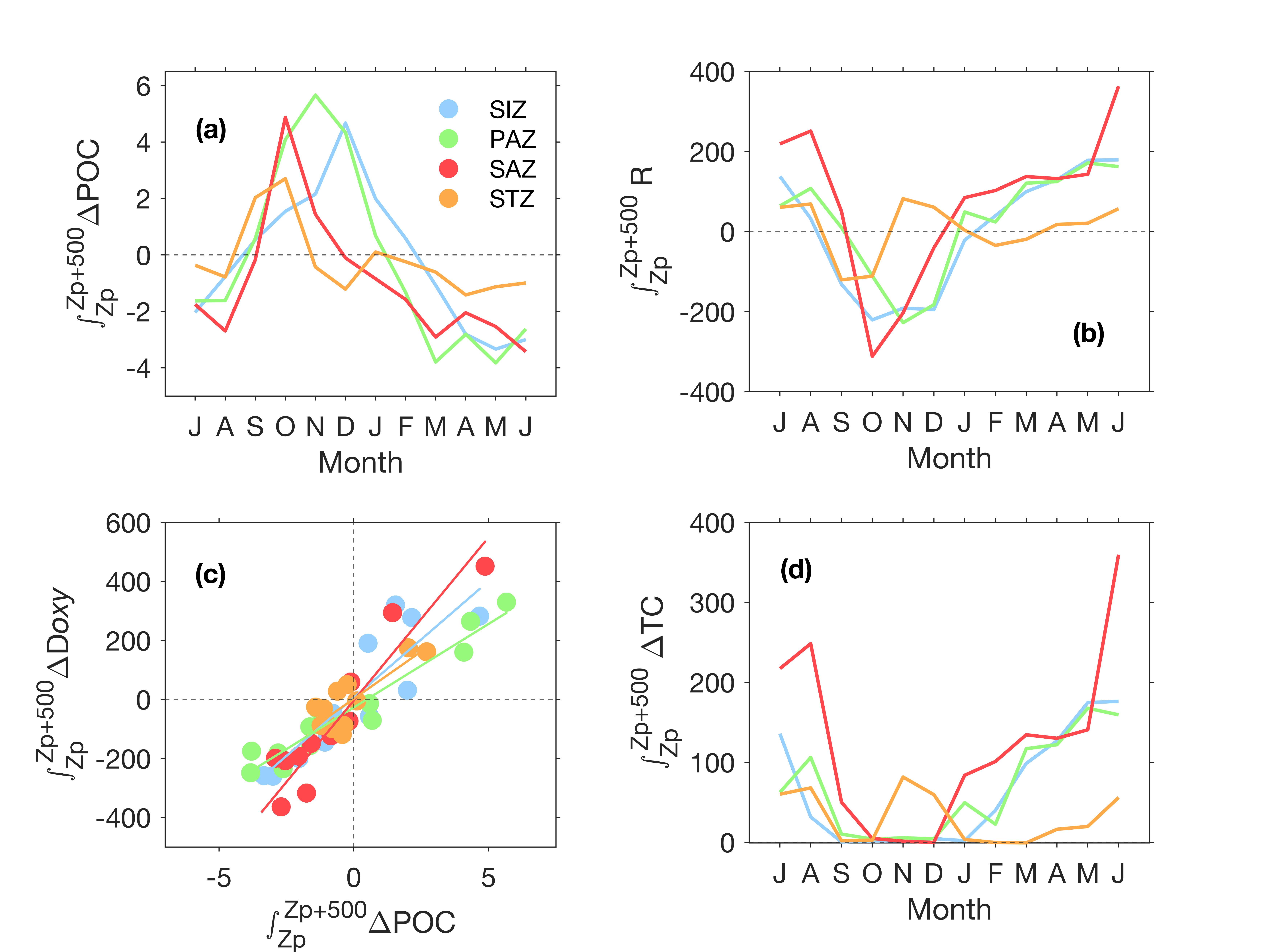
The marked seasonal succession in POC maxima at the ocean surface from north to south (STZ to SIZ, Fig. 3) translates into a similar seasonal succession for ∆POC from the export to the horizon depth (Fig. 5a; Supplementary Figure S5a). Our results show that temporal variability in POC represents a small proportion of the observed variability of TC, compared to respiration. However, respiration varies between zones and depths layers, as described below.
4.2 Heterotrophic respiration in the water column
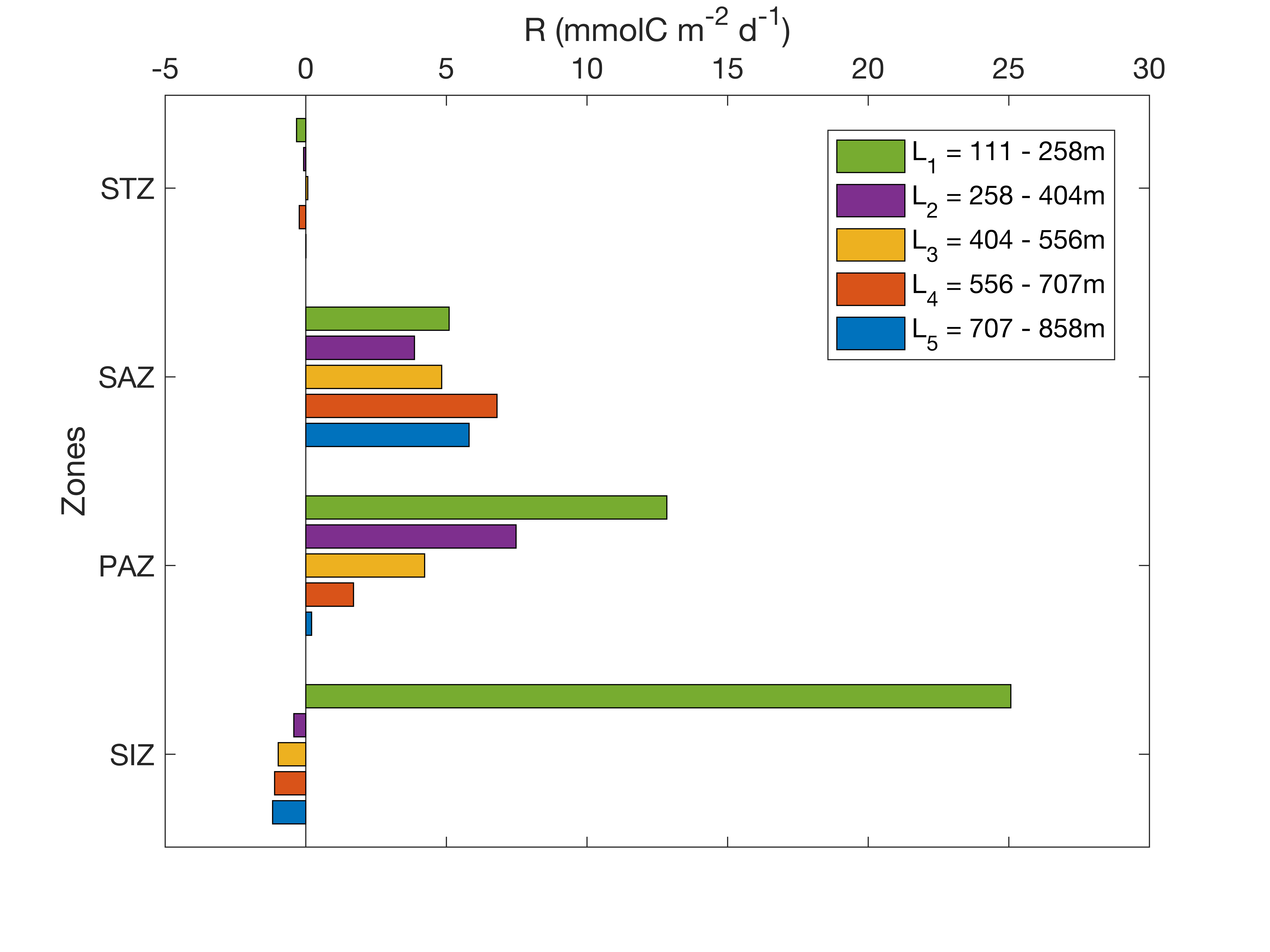
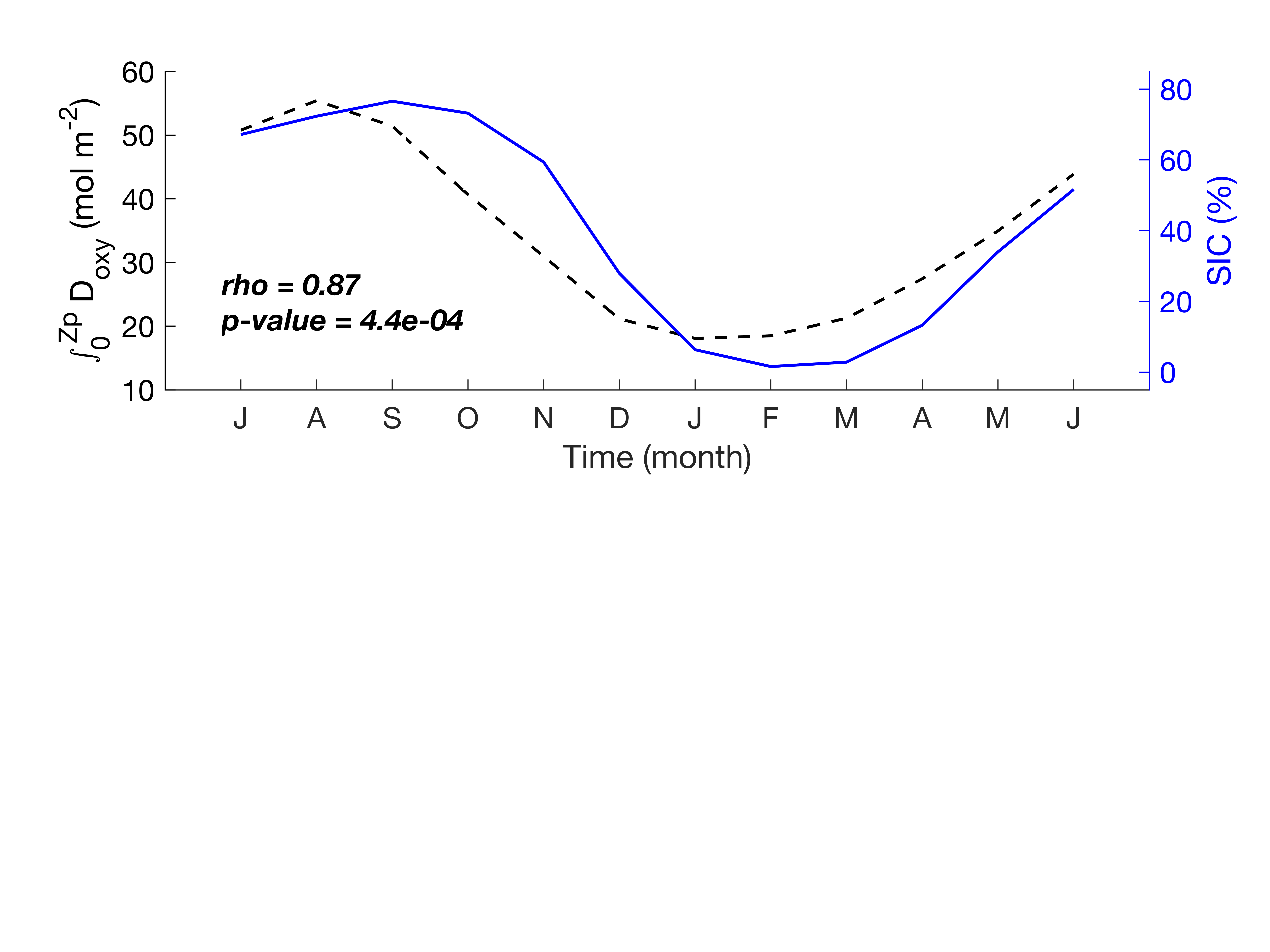
The highest respiration is observed in the SIZ (Fig. 7). Our results agree with Cardinal et al. (2005), who found that the highest respiration rate in the Indian sector was in the Antarctic zone compared to the SAZ and polar front. The SIZ and STZ, which are furthest apart, display the same behaviour in terms of horizon depth sensitivity (Supplementary Figure S2). Independent of the chosen export depth, estimates of integrated carbon export remain very similar from the surface to the deepest layers. This suggests that most of the respiration in the SIZ and STZ occurs below the productivity layer. In the SIZ, this is likely a direct response to the increased phytoplankton productivity when sea ice retreats (Fig. 3). Strong respiration was also reported during the sea-ice covered period (Briggs et al., 2018) from mid-June to December for a couple of floats. Our climatological estimations of integrated Doxy (surface to Zp) show similar results, where Doxy sharply decreases from August until December (Supplementary Figure S7). For comparison, strong remineralization was found in the top 250m in the Weddell Sea (Usbeck et al., 2002). The observed surface POC in the STZ are more consistent throughout the year and the highest respiration rate is also found directly under the productivity layer (Fig. 7). Several studies reported that in warm water conditions, respiration is enhanced (Cavan et al., 2019; Wohlers et al., 2009), and can respond twice as fast to increasing ocean temperature compared to photosynthesis (Boscolo-Galazzo et al., 2018). Combined with weaker seasonal variability, this might explain the relatively high subsurface respiration values in the STZ, although still lower compared to the SIZ where phytoplankton productivity and associated respiration is higher.
The vertical distribution of carbon export (TC) stands out in the PAZ and SAZ. In the PAZ, values converge at + 500m on average from Zp (Supplementary Fig. 2c), while the estimations increase with depth in the SAZ. This means that from + 500m, the remineralization from heterotrophs in the PAZ decreases, while it remains relatively constant with depth in the SAZ. A similar respiration rate at depth (Fig. 7, SAZ) can imply a constant transfer of POC through the water column, potentially via vertical export of zooplankton fecal pellets (Cavan et al., 2015; Le Moigne, 2019). Zooplankton usually migrate to the surface and feed at night to avoid predation, and defecate at deeper depths during the day (Steinberg & Landry, 2017), resulting in carbon transfer deeper in the water column and therefore deeper respiration. This transport of organic carbon by mesozooplankton usually represents less than 40% of the total POC flux (Turner, 2015). In addition, fecal pellets can be highly resistant to degradation (Riou et al., 2018; Tamburini et al., 2006), leading to high carbon flux and transfer in the water column. In this scenario, in the SAZ, the zooplankton migration and fecal pellets signals seem to dominate a more evenly distributed respiration signal throughout the mesopelagic layer (Fig. 8).
4.3 Perspective from previous studies
Compared to previous work related to annual net community production (ANCP), our estimates of carbon export are higher. Our values are close to those previously reported in the SAZ and STZ, but greater in areas of higher biological productivity, notably in the SIZ. Many approaches have been used to estimate carbon export and ANCP. Some studies looked at nutrient drawdown in the upper layer (Arteaga et al., 2019; Johnson et al., 2017b; Munro et al., 2015), but this technique does not account for nutrient replenishment from below (vertical mixing or advection) or heterotrophic activity within the mixed layer. Others quantified export below their defined productivity layer from sediment traps (Lourey & Trull, 2001; Pilskaln et al., 2004) which does not account for respiration. Both methods are likely to be prone to underestimation, as respiration can represent up to 90% of the export production in the mesopelagic zone (Jacquet et al., 2011). Thorium isotopes are also commonly used (Le Moigne et al., 2016; Planchon et al., 2013; Puigcorbé et al., 2017; Smetacek et al., 2012), accounting for all the POC exported from the surface waters.
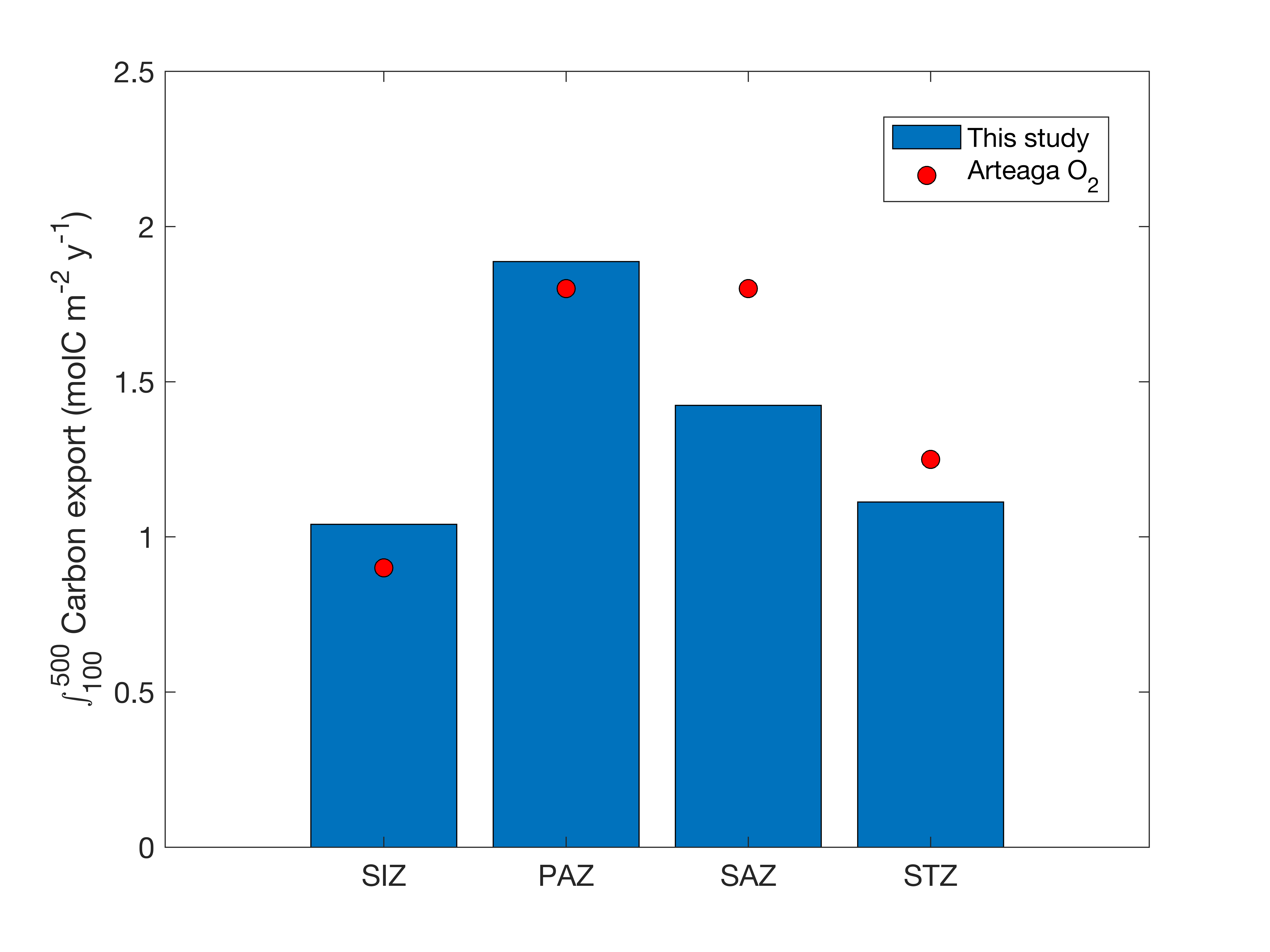
When we performed our calculations over 100-500m depth range like in Arteaga et al. (2019), we obtained very similar results (Supplementary Figure S8), because both methods rely on oxygen drawdown, but applied differently. Our estimates are 1.04, 1.89, 1.42 and 1.11 molC m-2 y-1 for SIZ, PAZ, SAZ and STZ respectively, compared to 0.9, 1.80, 1.80 and 1.25 molC m-2 y-1 for their study. Note that we binned their results in similar zones for comparison. This demonstrates the rigor of this new method to derive respiration from BGC-Argo floats.
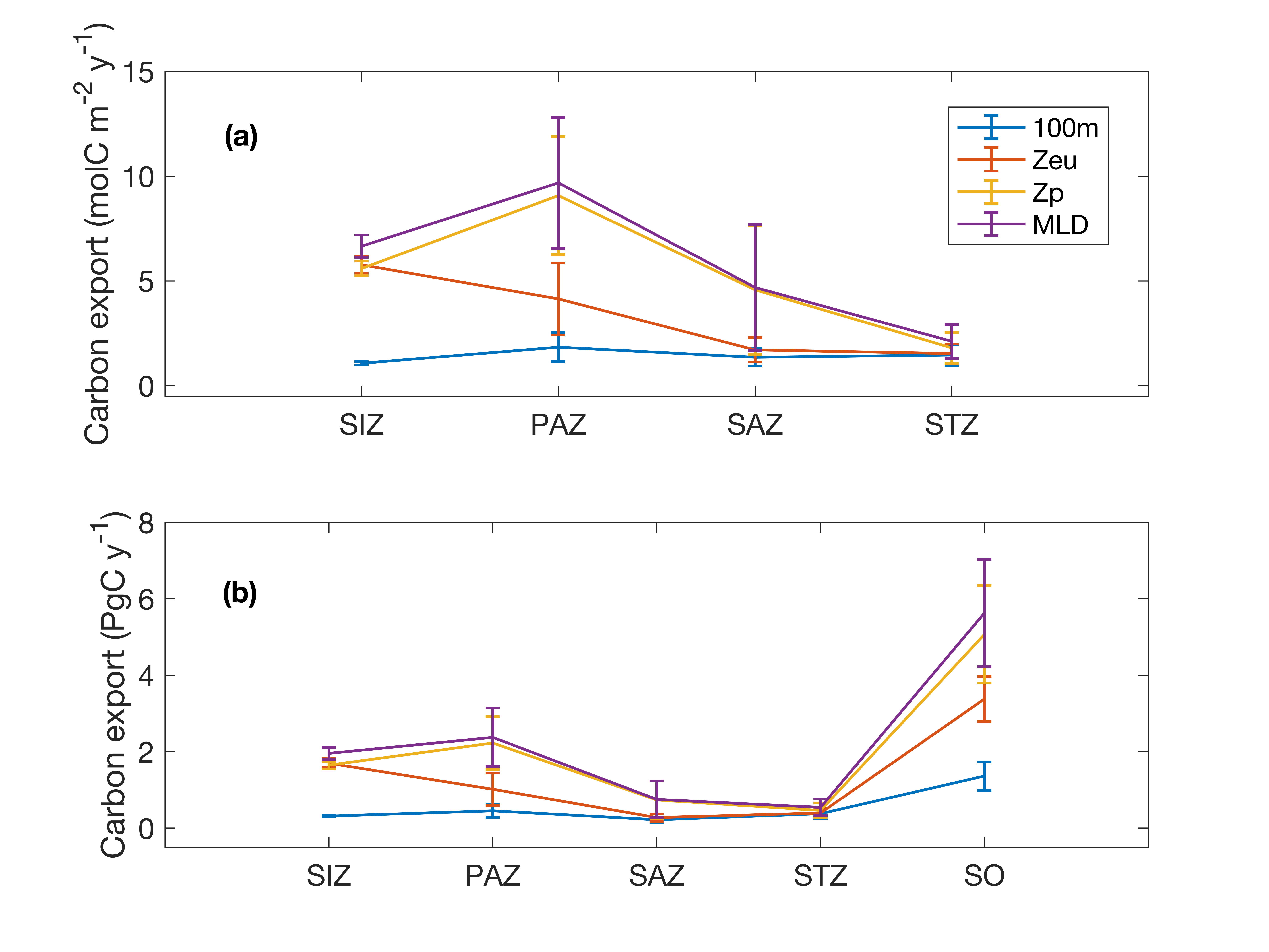
Our basin integrated calculation estimated a SO carbon export of 5.08 PgC y-1, which is higher than earlier values reported. However, most of the studies did not consider the SO to extend as far north as 30°S, or include the SIZ, or both. For example, the latest budget of 3.89 PgC y-1 calculated by Su et al. (2022) based on BGC-Argo floats observations did not consider the SIZ. If we remove the SIZ, our estimation falls to 3.4 PgC y-1, slightly smaller than their number, but still with some differences in zone definition and method used. Furthermore, the studies compared in Fig. 6b mostly defined the SO south of 40 or 50°S, discarding estimations from the STZ and some of the SAZ. Aside from the definition of regions, we argue that a basin scale calculation using all available floats allows for a better estimation of carbon export compared to studies relying on extrapolation of fewer data from restricted locations. In particular, our work provides a new and extended circumpolar SIZ estimate, an area which has been largely unstudied in the past because of the paucity of observational data under ice.
4.4 Uncertainties and caveats of carbon estimations
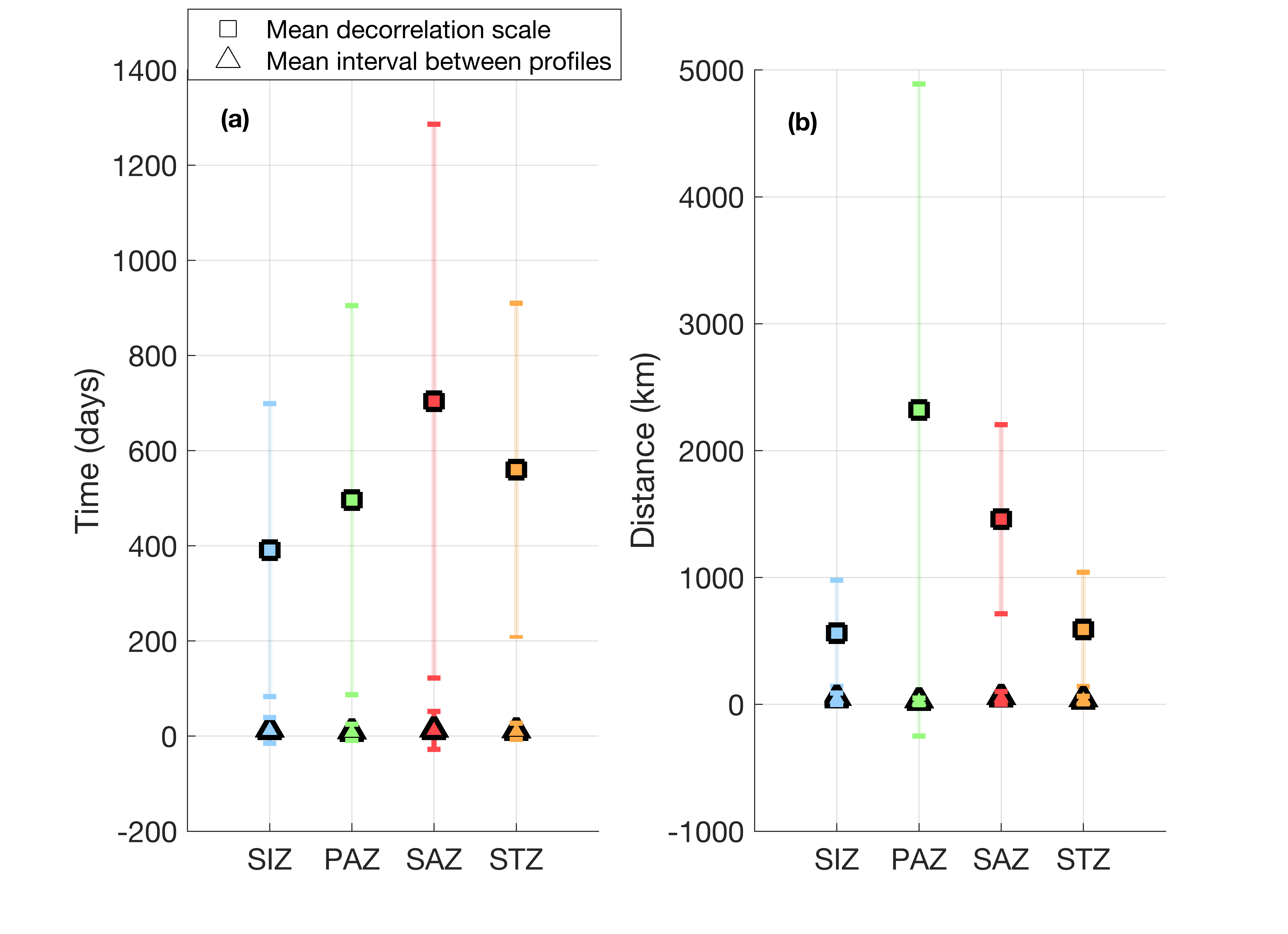
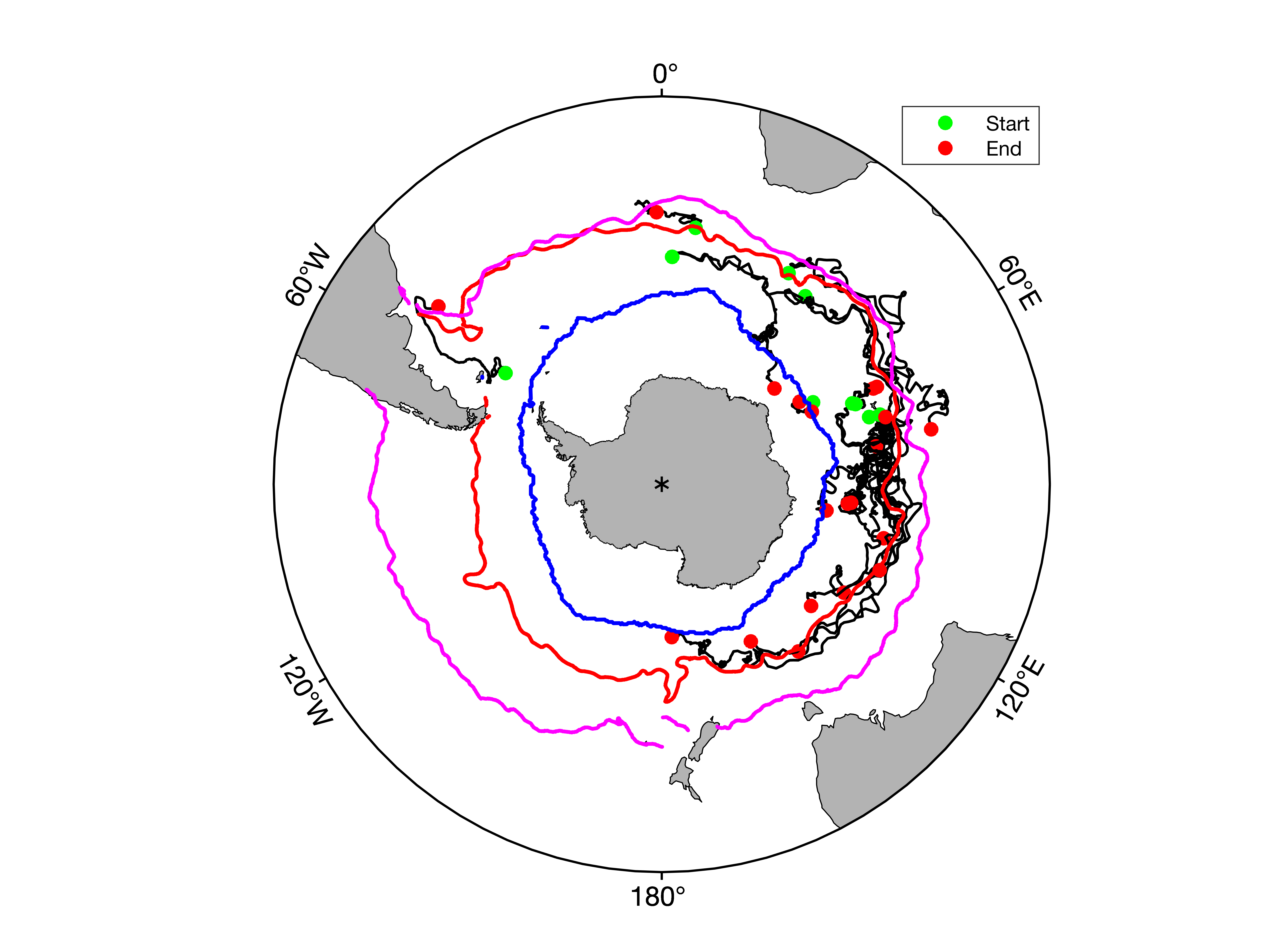
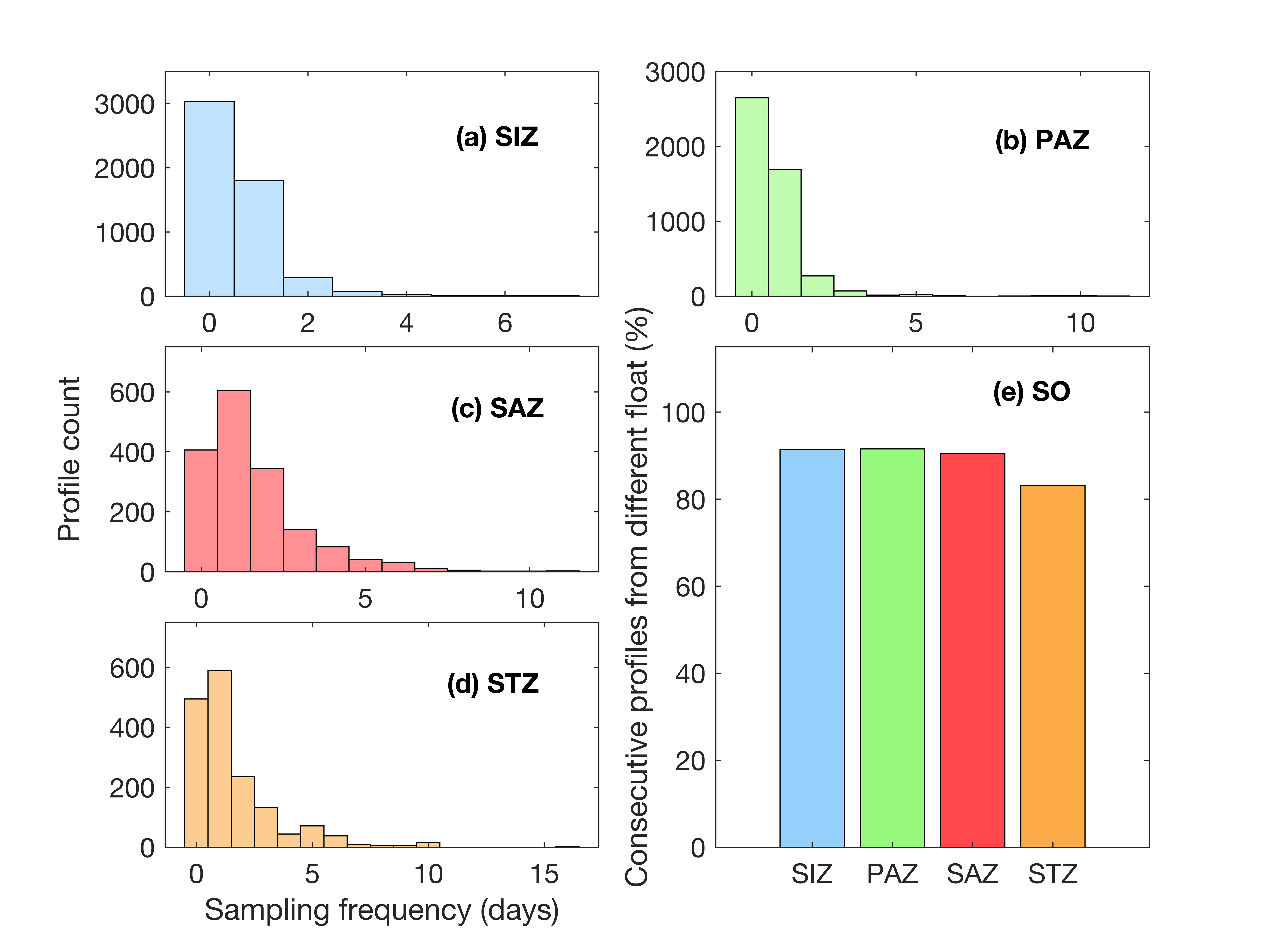
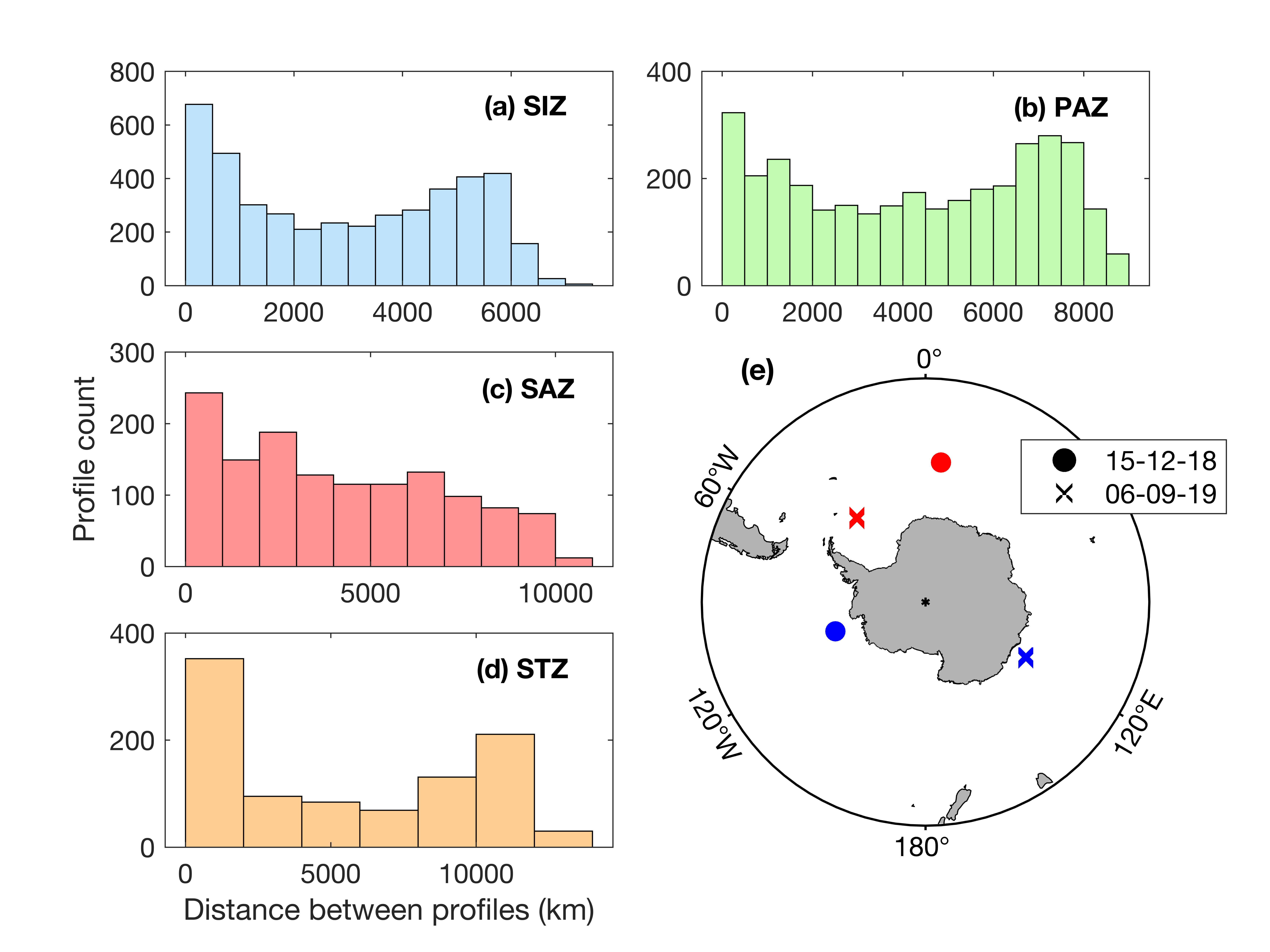
The primary goal of our study was to quantify the importance of the SIZ in the overall circumpolar SO carbon export. However, sea ice prevents floats from surfacing and transmitting their data in real time (Hague & Vichi, 2021; Riser et al., 2018). Therefore, it is not known if the spatial distances between consecutive profiles under ice are comparable to those in the open ocean. Large distances between profiles may bias our SIZ carbon export estimates compared to PAZ, SAZ and STZ, if the observed changes in POC or oxygen were due to spatial and not temporal variability. Only 0.2% of all SO pairs of profiles were separated by more than 300 km, which Argo-floats are primarily designed for (Fig. 8a; Riser et al., 2018). Consecutives pairs of profiles under sea ice were on average closer than in open water conditions in the SIZ (Figs. 8b-c). All the under-sea ice profiles are within a 150 km distance, while 99% of open water profiles are within that range. This confirms that the pairs of profiles used to derive our metrics of interest under ice are representative of processes within the same water masses. As well, the decorrelation scale was investigated. The average mean decorrelation scale in space and time showed to be greater than the mean space and time interval between profiles (Supplementary Figure S9). This implies that all consecutive pairs of profiles used to derive R and ∆POC likely capture the same water masses.
Sinking rate of POC depend on when or where iron is available in the Southern Ocean (Obernosterer et al., 2008), The SOIREE experiment reported sinking rates reaching 1.6m d-1, 2.5 m d-1 and up to 4 m d-1 in the SIZ following iron addition conditions (Boyd et al., 2000; Maldonado et al., 2001; Waite & Nodder, 2001). South of Tasmania, Cassar et al. (2015) described a sinking rate of 6 m d-1 on average, reaching a maximum of 19.5 m d-1. Fecal pellet sinking rates were also shown to be high in the SO, ranging from 82 m d-1 to 437 m d-1 north of the Antarctic Peninsula in the top 400m (Liszka et al., 2019). This wide range of sinking rates observed during ship-based campaigns imply that, over the 10 days sampling frequency by the BGC-Argo floats, large sinking events (and the associated respiration) may be missed.
To try to resolve this, we compared our carbon estimates (from the entire dataset) to estimates derived from SOCCOM floats only (10 days sampling interval), and SOCLIM and remOcean only (1 to 7 days sampling interval). Using SOCLIM and remOcean floats reduced our sample size by 75%, with very few SOCLIM/remOcean profiles in the SIZ and STZ compared to PAZ and SAZ (Supplementary Figure S10). Despite being higher, estimates of carbon export from only SOCLIM and remOcean floats, both in molC m-2 y-1 and PgC y-1, were not statistically different (Kruskal-Wallis; p-value > 0.1) from the whole array of BGC-Argo floats nor the SOCCOM floats array in the PAZ (13.02 vs 9.99 vs 10.77 molC m-2 y-1; 3.19 vs 2.45 vs 2.64 PgC y-1; Supplementary Table T1). However, in the other regions, the carbon export estimates from SOCLIM and remOcean were significantly higher than those from the all-floats and SOCCOM floats only arrays. So, when more profiles are used, the carbon export estimates between the three groups of floats are closer, as seen in the PAZ. Estimates from the SOCLIM and remOcean profiles in the SIZ, SAZ and STZ only have very few profiles that are spatially restricted to a small region in the Indian sector, compared to the PAZ profiles which show a better spatial coverage in the eastern SO. Therefore, we place higher confidence in our calculations using all floats and profiles, despite the lower sampling frequency of 10 days for the majority of them. This point of view is corroborated by Llort et al. (2018), who showed that SOCCOM floats can be used to capture fast sinking eddy-related carbon export episodes.
Another avenue to address the sampling frequency would be to merge profiles from all floats for a given province and derive parameters from the closest profiles in time. Opting for this method certainly allows for a greater sampling frequency compared to a usual 10-day window, from the same day to 2 days in most cases (Supplementary Figure S11a-b-c-d). However, this method implies that every calculation made from the closest time t1 to time t+ 1 can be performed on profiles from different floats that are in different areas, possibly different water masses, within the same zone. With this approach, about 90% of all consecutive profiles used to derive ∆POC and R are from different floats for the 4 zones (Supplementary Figure S11e), with significant spatial gaps (Supplementary Figure S12). Therefore, we believe that comparing consecutive profiles from a same float, and then averaging per month and zones, is the most suitable method for this study and to compare our results with past studies done using BGC-Argo floats.
Although we constrained physical fluxes using a strong salinity change criteria threshold, we make the assumption that physical fluxes are deemed negligible when deriving R (Ledwell et al., 1993), as previous studies did when deriving carbon export from oxygen (Arteaga et al., 2019; Hennon et al., 2016; Su et al., 2022). We however recognize that in reality, the hydrodynamics likely modify the local oxygen balance, therefore adding uncertainties. The method proposed by Arteaga et al. (2019) captured the special pattern of carbon flux in CM2-1 models, but underestimated the magnitude compared to the models. They suggested that this could be due to a mismatch between floats position and the lack of detritus flux in the gridded cell model. This implies that their observed estimates might be more representative of the ocean processes than the models, in respect to the natural spatial variability of carbon export in the SO. Oxygen from vertical and lateral advection captured from the floats are likely tied with biological activity, which is hardly distinguishable from the actual respiration rate used in our method. This also indicates that the true respiration rate would be closer to the ∆POC. Finally, lateral advection effect on oxygen concentration was investigated in the SO Indian and Pacific sector (Hennon et al., 2016) but did not show significant input.
Nevertheless, such processes have been shown to be significantly smaller than ANCP itself ( Arteaga et al., 2019; MacCready & Quay, 2001; Munro et al., 2015), or accounting for a very small fraction of change in Doxy (3% for advection in the SIZ, Briggs et al., 2018). Considering the floats as quasi-lagrangian and looking at large spatial and temporal scales (monthly variability) and averaging from an extended fleet could mean that smaller scale positive and negative changes in oxygen balance or cancel each other (Hennon et al., 2016; Martz et al., 2008; Najjar & Keeling, 1997). Another factor to consider is the calcium carbonate signal in the Great Calcite Belt (GCB), extending from 30° to 60°S. Balch et al. (2016) showed that bbp is high in this area due high particulate inorganic carbon (PIC) from calcification. Using our method, it is not possible to distinguish PIC from POC, so the presence of PIC likely causes some overestimation of POC. Methods have been developed to detect coccolithophore blooms using BGC-Argo floats (Terrats et al., 2020) based on bbp and chl-a. However, we argue this would likely have little effect on our carbon export estimation as (i) PIC was shown to have very little contribution to annual net community production compared to POC (Haskell II et al., 2020), (ii) high calcium carbonate production does not increase POC export (Balch et al., 2016) and (iii), most of the calcium carbonate is remineralized in the photic zone, therefore having little effect on export (Ziveri et al., 2023) and (iv) POC contributes very little to the total carbon export compared to respiration (Fig. 5d).