2.1. Experiment site and design
The field experiment started in April 2021 and finished in May 2022, on a vegetable field in Houxi Town, Xiamen city, with the coordinates 118º02′01.31′′ E, 24º38′16.93′′ N. With a temperate and wet climate, Xiamen is a part of the subtropical maritime monsoon climate region. The average annual temperature is around 20.8 °C, the average annual sunshine duration is approximately 2233.6 h per year, the average annual sunshine rate is about 51%, and the average annual rainfall is approximately 1200 mm (Fang et al. 2023). Vegetables and rice are the two main crops grown in Xiamen all year round because of the city's moderate temperature, ample sunshine, and plentiful rainfall. Typically, crops are grown all year long with several cycles, intense planting, and high fertilizer need. Brown sandy loam soil makes up the soil at the experiment location, and the fundamental physical and chemical characteristics of the topsoil (0–20 cm) before our cultivation experiment are bulk density 1.43 g cm-3, pH 4.56, maximum field water holding capacity 28.37%, soluble salt content 0.08%, ammonium N content 11.11 mg kg-1, nitrate N content 45.46 mg kg-1, organic matter content 13.6 g kg-1, total N 1.0 g kg-1, total potassium 1.8 g kg-1, total phosphorus 1.5 g kg-1, available phosphorus 110.2 mg kg-1, available potassium 287.5 mg kg-1, and soil particle composition of 0.04% clay, 21.95% powder, and 78.01% sand.
Chicken manure from the market was used in this experiment, because it is a common organic fertilizer that can be found in commercial organic fertilizer marketplaces in Xiamen, and around 60% of the farmers like to use chicken manure in leafy vegetable cultivation according to their planting experiences (Fang et al. 2023). Pyrolysis is a method which biochar is created by thermally carbonizing biomass in an oxygen-restricted environment inside of an airtight chamber. Biochar is a carbonaceous substance with a significant surface area, a porous structure, and an abundance of functional groups that is produced as a result of this thermochemical conversion, which is occasionally followed by functionalization and alterations (O’Connor et al. 2021).We pyrolyzed chicken manure for one hour at 500 degrees Celsius in an oxygen-limited environment to create biochar. Table 1 displays their physical and chemical characteristics.
|
Table 1: physical and chemical properties of chicken manure and CMB.
|
|
Organic fertilizer
|
Water content1(%)
|
pH2
|
TOC2 (%)
|
TN2 (%)
|
C/N2 (%)
|
TP2 (%)
|
TK2 (%)
|
|
Chicken manure
|
11.9±1.5
|
7.6±0.6
|
28.7±6.2
|
3.0±1.5
|
11.0±5.3
|
1.3±0.2
|
2.0±1.4
|
|
Chicken manure biochar
|
1.7±1.1
|
12.2±0.2
|
249.0±42.7
|
2.2±0.3
|
11.5±0.4
|
3.1±1.0
|
6.1±1.3
|
|
Notes: 1 Measured in wet matter. 2 Measured in dry matter. TOC (Total organic carbon); TN (Total nitrogen); TP (Total phosphorous); TK (Total potassium).
|
A field survey which was conducted on traditional crop cultivation and management (including NPK fertilizer types and application rate, organic and inorganic application ratio, substrate and chasing ratio) in four vegetable growing areas outside Xiamen Island from November 2020 to January 2021. The result showed that the application rates of N, P2O5 and K2O fertilizers for conventional leafy vegetables in Xiamen were 375, 225 and 263 kg ha-1, respectively, and the ratio of substrate to chase fertilizer was 6:4 for N fertilizer, and the average ratio of organic and inorganic N fertilizer application was about 3:7 (Fang et al. 2023).
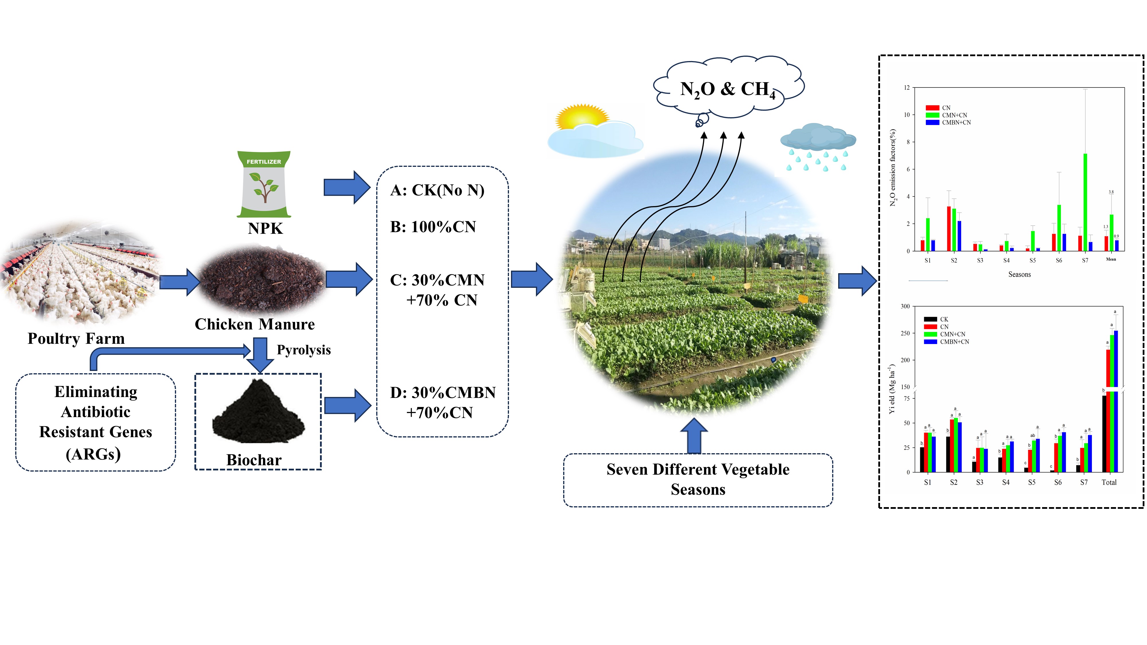
Based on aforesaid survey result, four treatments were set up in this field experiment: N-free control (CK); Conventional 100% chemical fertilizer N (CN); Conventional 30% chicken manure N (4.2 t ha-1) plus 70%CN (CMN+CN); 30% Chicken manure biochar N (5.2 t ha-1) plus 70% chemical fertilizer N (CMBN+CN). Three replications, 12 plots, plots size 2.5m×8.0m (20 m2), containing a planting size of 1.7m×8.0m (13.6 m2) were arranged in randomized group. Before the experiment began, a 50 cm wide by 0.8 mm thick plastic film was pre-buried between adjacent plots and replicates to stop inter-plot water and fertilizer interactions.
Two common leaf vegetables (pakchoi and swamp cabbage) are cultivated during this study. From April 2021 to May 2022, a total of 13 months, we carried out field cultivating experiments for seven different seasons: (S1) pakchoi (April 9 to May 8, 2021); (S2) swamp cabbage (June 15 to August 30, 2021); (S3) pakchoi (September 2 to September 28, 2021); (S4) pakchoi (October 13 to November 10, 2021); (S5) pakchoi (December 2, 2021 to January 11, 2022); (S6) pakchoi (January 29 to March 14, 2022), and (S7) pakchoi (April 10 to May 8, 2022). Pakchoi only grows for a short time about 28 days during the warm months of March through November and 40 days during the cold months of December through February of the following year. The growing cycle of swamp cabbage takes about 75–80 days. Pakchoi seed is spread out across each plot at a rate of 42 g in the first season and 33 g in the next. An experienced farmer uniformly distributes pakchoi seeds into each plot before incorporating them into the earth using a plow. With a density of 12 plants per square meter, swamp cabbages are transplanted with seedlings from the nearby farmer's fields.
For N, the basal dressing to top dressing ratio is 6:4. Based on 30% of the N application quantity (or 112.5 kg N ha), the precise amount of various organic compounds is applied is computed. Urea (N 46.0%), super phosphate (P2O5 12.0%), and potassium sulfate (K2O 50.0%) make up the chemical fertilizers used. In order to meet the required P/K dosage, more single super phosphate or potassium sulfate added to organic fertilizer if its P or K content falls below 98 kg P ha-1 or 218 kg K ha-1. All treatments received the same amount of phosphorus and potassium fertilizer applied to leafy vegetable in Xiamen, and totally used as basal fertilizer before planting. Irrigation, weeding, and other cultivating management techniques are carried out in accordance with regional customary norms and remain constant across various treatments. The irrigation equipment employed is a vertical rotating sprinkler system, and each treatment receives the same quantity of irrigation. According to farmers' experience, irrigate once after topdressing the soil surface with urea and irrigated once a day during rainless period when the soil surface appears to be dry and irrigated twice if the soil surface temperature is too high for vegetables in summer season. Typically, pesticides were applied once to twice during the growing season for vegetables.
At each harvest season, the biomass of the plants' above-ground parts in a 1 m × 1 m (1 m2) region from each plot is harvested and weighed. The fresh weight of the above-ground biomass is referred to as crop yield. Due to the swamp cabbage's lengthy growth cycle, the above-ground stems and leaves are harvested three times in 2021 on July 18, August 2, and August 30 and the yield is calculated as the total of the three harvests.
2.2. Sample collection and measurement method of greenhouse gases
GHGs emissions were measured in every plot from April 2021 to May 2022, in all seven vegetables growth seasons. Emissions were measured manually using closed static chamber method which was explained with details in other studies (Zheng et al., 2008; Gao et al., 2014). Each chamber was compost of a stainless-steel frame with a water-filled groove on top which sealed the upper chamber with a diameter of 40 cm and a height of 30 cm. To reduce the rise in air temperature, an insulating material was placed over the upper chamber. The frames remained in place for the whole of a crop growing season after being placed 10 cm into the soil. A total of four gas samples were collected during chamber closure at intervals of 10 minutes using 60 ml plastic syringes through a three-way stopcock and a Teflon tubing attached to the chamber. The initial sample was collected right after enclosure. After each basal-dressing and top-dressing fertilization, emissions of N2O and CH4 were measured once in every two days for 10 days and once in every 4 days for regular days. Between 9:00 and 11:30 am, measurements were done.
Gas chromatograph (GC, Agilent 7890, USA) equipped with electron capture detector (ECD) operating at 330 °C for N2O concentration and flame ionization detector (FID) operating at 250 °C for CH4 concentration was used to examine the concentrations of N2O and CH4 which is explained with details in another study(Li et al. 2023b).
The N2O and CH4 fluxes were calculated using the following equation:
F = k1 × P0 / P × 273 / (273 + T) × M / V × H × dc / dt
Where F (µg N m-2 h-1or µg C m-2 h-1) is N2O fluxes; k1 is a coefficient (0.001) for dimensional conversion; P0 (hPa) is the atmospheric pressure in the chamber which was assumed to not differ substantially from P (1013 hPa) which is the standard atmospheric pressure at the experimental site; T (°C) is the average air temperature in the chamber during the enclosure; M (28 g N2O-N mol-1) is the molecular weight of N2 in the N2O molecule; V (L mol-1) is the molecular volume at 1013 hPa and 273 K, H (m) is the chamber height; c (µL L-1) is the concentration of N2O; t (h) is the chamber enclosure time; dc / dt (µL L-1 h-1) is the rate of increase in N2O concentration in the chamber (Zheng et al. 2008; Gao et al. 2014). The fluxes of three replications for each measurement period were averaged to get the mean N2O and CH4 emissions. The arithmetic means of the two days that were closest to the days without measurements were used to estimate the N2O and CH4 fluxes for those days. The total N2O and CH4 emissions for each vegetable growing season were then calculated by adding the daily estimations. To find N2O Emission factor (EF) from our vegetable field, the amount of emitted N2O-N per kg N fertilizer was measured.
2.3. Soil sampling and measurements
Soil samples were taken during each vegetable crop season from each plot once every two days for ten days after each fertilization, and once every eight days on regular days, to determine soil moisture and soil mineral N (Nmin, NH4+-N + NO3−-N). A 3-cm-diameter gage auger was used to collect a depth of 20 cm soil samples. Soil samples were transported to laboratory in an ice box and immediately frozen at -18before extract soil Nmin. a 20 g soil sample was oven-dried to a constant weight at 105 ℃ to determine soil water content, and to calculate water filled pore space (WFPS) using the equation described in (Gao et al. 2014). A 12 g of fresh soil samples were weighed in a 200 ml plastic bottle, 100 ml of a 1 mol L−1 Potassium chloride (KCl) solution was added, and the mixture was shaken at 180 r for 1 hour before filtering. The extracts were stored at -18 ºC prior to analysis of NH4+-N and NO3−-N using a SEAL Analytical Auto Analyzer 3 (AA3, SEAL Analytical GmbH, Germany).
2.4. Determination of temperature and precipitation
Digital thermometer was used to measure the ambient temperature and the soil temperature at a depth of 10 cm during this study. The recorded ambient temperature and soil temperature as shown in Fig. 1. The air temperature in the headspace of the chambers were measured at the start and end of gas sampling using digital thermometers. The mean value represents the temperature during gas sampling and it was further used to calculate the GHG fluxes. And precipitation data were recorded by an automatic weather station at the experimental site as shown in Fig. 2.
2.5. Analysis of the relationship between N2O emissions and temperature and soil moisture
The links between N2O emission, temperature, and soil moisture were analyzed using the group mean value and the boundary line method (Schmidt et al., 2000). Refer to(Gao et al., 2014) for more information about this approach. When analyzing relationships among various parameters, the usage of group mean values has multiple advantages, including data conclusion, outlier reduction, statistical power increase, result comparison, and improved communication of study findings (Schmidt et al. 2000).
2.6. Statistical analysis
To evaluate the statistically significant differences in indicators among crop yields of various treatments at the 5% level (P < 0.05), SPSS 25.0 statistical software (IBM, Armonk, NY, USA) was used for data analysis. To create the necessary statistical analysis charts, SigmaPlot version 14.0 software (Inpixon, Palo Alto, CA) was used.