Study area and data
Hangzhou is located on the east coast of China, the capital of Zhejiang Province, between 29°11′-30°34′ N and 118°20′-120°37′ E (Fig. 10). Hangzhou has a subtropical monsoon climate with an average annual air temperature of 18.5°C and precipitation of 1,456.6 mm in 2022. Hangzhou is one of the four cities in China that are referred to as “hot stoves” due to their high summer temperatures. Summer in Hangzhou lasts from mid-June to late September 69. The average temperature during the summer in 2022 was 28.9°C. The Shangcheng, Gongshu, Xihu, Binjiang, Xiaoshan, Qiantang, Linping, Yuhang, and Fuyang districts of Hangzhou were selected as the main construction areas of the CI network.
The data used in this study mainly include remote sensing image, land cover, buildings, elevation and meteorological stations data, and the specific sources and descriptions are listed in Table 2.
Table 2
Data sources and description.
|
Data type
|
Source
|
Description
|
Resolution
|
Date
|
|---|
|
Remote Sensing data
|
https://www.gscloud.cn/
|
Landsat8/9 OLI/TIRS
|
30 m
|
2019–2022
|
|
Building data
|
https://map.baidu.com/
|
Building outline, height
|
-
|
2019
|
|
Land cover data
|
www.resdc.cn
|
6 primary and 25 secondary types
|
30 m
|
2020
|
|
Digital Elevation Model
|
https://www.gscloud.cn/
|
ASTER GDEM
|
30 m
|
2020
|
|
Meteorological data
|
rp5.ru
|
Wind direction and velocity
|
-
|
2019–2022
|
LST
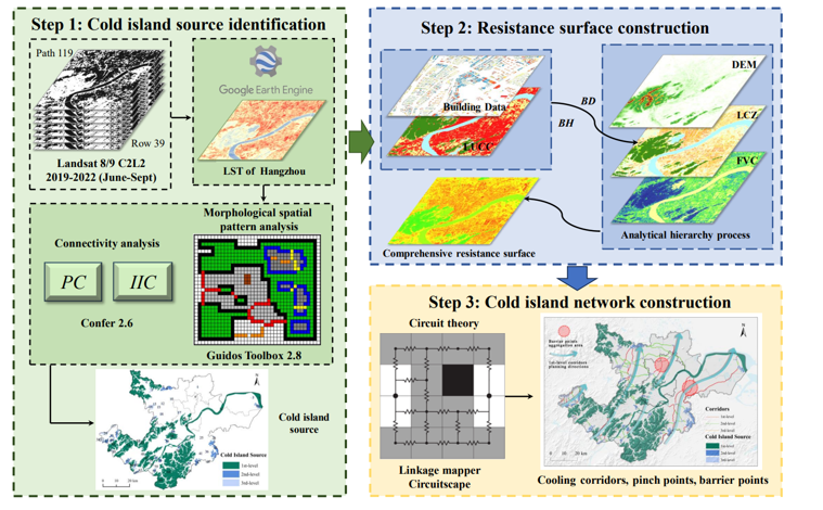
Landsat 8 and 9 C2L2 products were accessed on the Google Earth Engine (GEE) platform to obtain LST data and calculate the fractional vegetation cover (FVC). To avoid interference by extreme weather and better reflect the average LST in Hangzhou throughout the summer. We selected a total of 7 images (strip numbers Path 119, Row 39 and less than 10% cloud cover) taken during the summer months of 2019–2022 that cover the entire study area (Supplementary Table 2). The images were first de-clouded and then mean-synthesized. Finally, using the mean-standard deviation method to reflect the thermal environment pattern of the urban surface, the LST of Hangzhou was categorized into five thermal classes (Table 3) and below the medium temperature areas were defined as CI regions, whereas the other areas were defined as non-CI regions.
Table 3
LST classification level table.
|
LST Level
|
Grading Method
|
Value Range
|
|---|
|
Low Temperature area
|
\(\text{T} \le A -1.5 std\)
|
≤ 36.61°C
|
|
Sub-low Temperature area
|
\(A\)-1.5 \(std\) < T ≤\(A\) -0.5 \(std\)
|
31.61°C-36.05°C
|
|
Medium Temperature area
|
\(A\) -0.5 \(std\) < T ≤\(A\) +0.5 \(std\)
|
36.05°C-40.48°C
|
|
Sub-high Temperature area
|
\(A\) +0.5 \(std\) < T ≤\(A\) +1.5 \(std\)
|
40.48°C-44.92°C
|
|
High Temperature area
|
\(\text{T} > A +1.5 std\)
|
> 44.92°C
|
T is the LST value, \(A\) is the mean (\(A\) = 38.27°C), and \(std\) is the standard deviation (\(std\) = 4.44°C).
CI source identification
We utilized MSPA, which is a mapping algorithm based on mathematical morphology 70. This method automates the categorization of the pixel data (binary raster images) of the focal feature classes into new structurally connected feature classes at the image-element level 71. It is commonly used to characterize the geometric features, patterns, and connectivity of images. Using the MSPA method, CI patches that play important roles in the regional LST landscapes can be identified. In our study, LST maps were first reclassified by setting the CI regions into the foreground, and the non-CI regions into the background. Then, MSPA classification was performed on the binary images using Guidos Toolbox 2.8 software, with the default 8 neighborhood rule with a width of 1. This method further classified CI areas into seven CI patch landscape types: core, bridge, branch, islet, loop, perforation, and edge. Among them, core has been shown to be the most important type in the spatial pattern of urban CIs28.
The landscape connectivity index can quantitatively characterize the degree to which the landscape promotes or hinders the movement of substances between patches, allowing the identification of CI patches with greater connectivity. Based on the extracted MSPA core types, we selected CI patches larger than 1 km² as CI sources. The probability of connectivity (PC) and index of connectivity (IIC) indices were chosen to measure the magnitude of connectivity of each CI source. The PC and IIC were calculated using Confer 2.6 software. By calculating and comparing the number of links, components, IIC-equivalent connectivity, and PC-equivalent connectivity at different distance thresholds 56, we found that the indices achieved the best results when the distance threshold was 1,200 m (Supplementary Fig. 2). The connectivity probability was taken as 0.5, and the PC and IIC were calculated as follows:
$$PC=\frac{{\sum }_{i=1}^{n}{\sum }_{j=1}^{n}{a}_{i}\times {a}_{j}\times {{P}_{ij}}^{*}}{{A}_{L}^{2}}$$
1
$$IIC=\frac{{\sum }_{i-1}^{n}{\sum }_{j-1}^{n}\frac{{a}_{i}{a}_{j}}{1+n{l}_{ij}}}{{A}_{L}^{2}}$$
2
where \({A}_{L}\) is the overall area of the CI sources, \(n\) is the overall number of patches on the CI sources layer L,\({a}_{i}\) and \({a}_{j}\) are the areas of CI sources patches \(i\) and \(j\), and \({{P}_{ij}}^{*}\) is the probability of the maximum connection between CI sources patches \(i\) and \(j\).
The PC value can be taken to evaluate the intensity by which the cooling effect of the CI source. Those with PC > 2 were selected as strong CI sources and those with PC < 2 as weak CI sources. Meanwhile, IIC > 0.2 was regarded as a CI source with strong connectivity, and IIC < 0.2 was regarded as a CI source with weak connectivity. Finally, CI sources with a good cooling effect and strong connectivity were designated as 1st-level CI sources, those with a poor cooling effect and weak connectivity were classified as 3rd-level CI sources, and the remainder were classified as 2nd-level CI sources.
LCZ Classification
Each LCZ type contains different land cover, surface, and human activity features. We classified LCZ types based on a 30 m grid using land cover data combined with building data, and building-type LCZs were determined by calculating building height and density (Supplementary Table 3), while nature-type LCZs were determined based on secondary land cover data 52. The classification criteria are shown in Table 4.
Table 4
|
LCZ
|
Description
|
LCZ
|
Description
|
|---|
|
LCZ1
|
Compact super high-rise
(Over 12 floors)
|
LCZA
|
Dense trees
|
|
LCZ2
|
Compact high-rise
(10–12 floors)
|
LCZB
|
Scattered trees
|
|
LCZ3
|
Compact middle-high-rise
(7–9 floors)
|
LCZC
|
Bush, scrub
|
|
LCZ4
|
Compact mid-rise
(4–6 floors)
|
LCZD
|
Low plants
|
|
LCZ5
|
Compact low-rise
(1–3 floors)
|
LCZE
|
Bare rock or paved
|
|
LCZ6
|
Open super high-rise
(Over 12 floors)
|
LCZF
|
Bare soil or sand
|
|
LCZ7
|
Open high-rise
(10–12 floors)
|
LCZG
|
Water
|
|
LCZ8
|
Open middle-high-rise
(7–9 floors)
|
LCZ1-5 BD ≥ 0.4
LCZ6-10 BD < 0.4
|
|
LCZ9
|
Open mid-rise
(4–6 floors)
|
|
LCZ10
|
Open low-rise
(1–3 floors)
|
Resistance surface construction
Constructing the resistance surface is a key step in building a CI network that reflects the magnitude of thermal resistance of CI sources during the cooling process. Based on the methods used in related studies, the LCZ, FVC, and DEM were selected to build the resistance surface (Table 5) 66,40,56. The LCZ contains building density, building height, and land use information, which can effectively reflect the 3D impact within urban buildings on CI diffusion compared to land use data alone. Different LCZ types have considerable surface temperature heterogeneity, and building-type LCZs generally have higher temperatures than nature-type LCZs. Therefore, the corresponding resistance value was assigned according to the LST height of the LCZ. Furthermore, the FVC and DEM values are negatively correlated with the LST, thereby affecting CI diffusion. For example, the greater the FVC, the lower the LST and the smaller the resistance value. The FVC was obtained using annexed Equation A1and A2. High elevations typically have relatively higher wind speeds and air mobility, which are favorable attributes for cold source diffusion 42. The resistance of the LCZ, FVC, and DEM was assigned a value between 0 and 100 56, and the weight of each factor was identified through the Analytical Hierarchy Process (AHP) 40,54. The factors were weighted using the integrated resistance raster map of CI diffusion in Hangzhou, which was obtained by superimposing the factors by weight (0.7306, 0.1184, and 0.0810 for LCZ, FVC, and DEM, respectively.
Table 5
Resistance factors and classification.
|
Resistance Index
|
Weight
|
Class
|
Value
|
Resistance Index
|
Weight
|
Class
|
Value
|
|---|
|
LCZ
|
0.7306
|
LCZ1
|
42
| | |
LCZE
|
48
|
|
LCZ2
|
78
|
LCZF
|
18
|
|
LCZ3
|
84
|
LCZG
|
0
|
|
LCZ4
|
90
|
FVC (%)
|
0.1884
|
< 10
|
90
|
|
LCZ5
|
96
|
10–30
|
70
|
|
LCZ6
|
36
|
30–50
|
50
|
|
LCZ7
|
60
|
50–70
|
30
|
|
LCZ8
|
66
|
≥ 70
|
10
|
|
LCZ9
|
72
|
DEM (m)
|
0.0810
|
0–59
|
90
|
|
LCZ10
|
54
|
59–173
|
70
|
|
LCZA
|
6
|
173–312
|
50
|
|
LCZB
|
24
|
312–507
|
30
|
|
LCZC
|
12
|
507–1078
|
10
|
|
LCZD
|
30
| | | | |
CI network construction
We used CT to identify cooling corridors between CI sources, which were constructed in ArcCatalog by invoking the Build Network and Map Linkages function in the Linkage Mapper Tools. McRae72 first to proposed application of CT to ecology, which utilized the property of electrons randomly traveling in circuits to model species migration or ecological flow. As shown in Fig. 12, in this study, each CI source considered as a circuit node, the comprehensive grid resistance surface was regarded as the resistive surface through which electrons flow, and the minimum resistive cost distance path through which the two CI sources were connected was regarded as the cooling corridor. In each pair of circuit nodes, one node was connected to a 1 A current and the other node was grounded. The effective resistance values between multiple pairs of circuit nodes were iteratively calculated 28. The cumulative current value represents the net movement to a destination node. A cooling network connecting the CI source was constructed by simulating the cyclic process of the random motion of electrons through the CI source.
Cooling corridors were graded according to the direction of the prevailing summer winds and length. First, corridors less than 1 km were categorized as 3rd-level. Corridors under the non-dominant wind direction were categorized as 2nd-level. Corridors under the dominant wind direction were categorized as 1st-level. Then, the pinch and barrier points were further localized through the use of Circuitspace software and the Linkage Mapper Tools. Pinch points are an important component of a CI network and are the best cooling areas in the cooling corridors, which manifest in the circuit network as specific areas with the highest cumulative current density values. Pinch points are identified using the ‘all to one’ mode in the Pinchpoint Mapper tool. Barrier points are heated spaces that block the connection of CIs and are represented in the circuit network by areas with the highest cumulative current recovery values. Using the Barrier Mapper tool, barrier points were identified within a search radius of between 30 and 120 m 66. By protecting the pinch points and eliminating the barrier points, the connectivity between the CI sources can be enhanced, which improves the structure of the CI network and substantially reduces the UHI effect.