Resource population and phenotypes collection
Simmental beef cattle (born between 2008-2015) were established in Ulgai, Xilingole League, Inner Mongolia of China. Six body size traits at three growth stages (6, 12, and 18 months after birth) were measured simultaneously for each individual, and blood sample specimens were collected during the regular quarantine inspection of the farms was conducted. All procedures were conducted in strict compliance with the guidelines established by the Ministry of Agriculture of China. Some descriptive statistics and heritability estimates of six traits at three growth stages are presented in Table 1.
Genotyping and quality control
Genomic DNA was isolated from blood samples using the TIANamp Blood DNA Kit (Tiangen Biotech Co.Ltd.,Beijing, China). DNA quality was acceptable when the A260/A280 radio was between 1.8 and 2.0. Genotyping was performed with the Illumina BovineHD Beadchip (Illumina Inc., San Diego, CA, USA) and the PLINK v1.07 Software was used for quality control [60]. In this study, animals with a call rate (0.9) were discarded. SNPs were deleted the following standards, including minor allele frequency (0.01), SNP call rate (0.05) and Hardy-Weinberg equilibrium values (p110−6). Finally, 671192 SNPs on 29 autosomal chromosomes with an average distance of 3 kb were generated for the analysis.
Single‑trait GWAS
We used the compressed mixed linear model (CMLM) for single-trait GWAS because it reduced computing time by clustering individuals into groups, increased the power in QTN detection by eliminating the need to re-compute variance components, and enhanced the effectiveness in correcting the inflation from the polygenic background and controlling the bias of population stratification [61, 62]. Briefly, a principal components analysis (PCA) was performed and a kinship matrix was calculated using the Genome Association and Prediction Integrated Tool (GAPIT) package in R v3.4.2 [63]. To revise the effects of population structure, the Q matrix was reflected by the PCA. To replace the incomplete genealogy, the K matrix was calculated by the VanRaden algorithm [64]. This model is as follows:
y = W υ + X+ Z u + е
where y is a vector of the observed phenotypes; W was a vector of SNP genotype indicators, which was coded as 0, 1 and 2 corresponding to the three genotypes AA, AB, and BB with B being the minor allele. υ was the effect of marker, which is treated as a fixed effect; Variable is an incidence matrix for non-genetic fixed effects, and is a non-genetic vector of fixed effects including month ages (time of birth to measurement), enter weight (weight of just entering the farm), fattening days (time of entering farm to measurement) and principal component effects (the top three eigenvectors of the Q matrix). Variable Z is an incidence matrix for a vector of polygenic effects, and parameter u is a vector for residual polygenic effects with an assumed N (0, Kσ2) distribution, where σ2 is the polygenic variance and K is a marker inferred kinship matrix. While е is a vector for random residual errors with a putative N (0, I) distribution, where is the residual variance. The CMLM analysis was performed with GAPIT Software package (http://www.maizegenetics.net/gapit). Quantile–quantile (Q–Q) plots were generated to visualize the goodness of fitting for the GWAS model accounted by the population structure and familial relatedness. The negative logarithm of the p value from the model was calculated against the expected value based on the null hypothesis. The threshold p value after Bonferroni correction was 0.05/N = 7.45×10⁻⁸, where N is the number of SNPs. In light of the fact that the Bonferroni correction results were too stringent with low statistical power [65]. Hence, we adopted the false discovery rate (FDR) to determine the threshold values for Single-GWAS, Multi-trait GWAS and LONG-GWAS. The FDR was set as 0.01, and the threshold p value was calculated as follows:
P = FDR n/m
where n is the number of P<0.01 in the results, and m is the total number of SNPs [66].
Multi‑trait GWAS
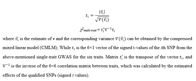
The multi-trait GWAS were conducted to detect pleiotropic SNPs and the model was a Chi square statistic, which approximately followed a Chi square distribution with the number of traits tested as the number of degrees of freedom. It was calculated for each SNP using the following formula [67]: (see Formula in the Supplementary Files)
LONG-GWAS
Information on body size traits at three growth stages were obtained from all individuals, and we conducted a longitudinal GWAS by LONG-GWAS [68]. This model was similar to CMLM, except that the phenotypic variance was partitioned to SNPs, fixed factors (the above-mentioned vector), polygenic effects, time stage effects and residual variance. Moreover, numerous studies have reported that the longitudinal design could facilitate the identification of time-dependent and consistent loci, which increased the statistical power due to their effectiveness in incorporating the correlation structure of multiple measurements and alleviating the multiple testing burden [26, 27, 69]. The code data implementing this method may be found at http://genetics.cs.ucla.edu/longGWAS/. This model is as follows:
= Wv + Zu ++ e
In this formula, is the adjusted phenotype. The incidence matrix W, Z, the vector v, u and e are consistent with CMLM mentioned above. Differently, the parameter is a vector for time stage effects with a putative N (0,) distribution, where D is a known block diagonal matrix representing the covariance between permanent environmental components. The D matrix was calculated by this formula: D= E ⊗ I, where E is a 3 × 3 matrix representing the covariance between the set of 3 time points for each individual.
Identification and annotation of candidate genes
The UMD3.1 genome assembly was used to located genes for annotation, and the QTLdb database (http://www.animalgenome.org) was applied to search for related QTL regions.