Study cohort
This study was retrospective and approved by Institutional Review Board (protocol 2019-SR-396) of the first affiliated hospital with Nanjing Medical University (NUH) and need for written informed consent was waived. All procedures performed in studies involving human participants were in accordance with the 1964 Helsinki declaration and its later amendments.
The primary patients comprised of an evaluation of two collaborative centers’ database (Center 1, NUH; and Center 2, the first affiliated hospital with Soochow University [SUH]) for medical records and were histologically proven between January 2014 and December 2019. The inclusion criteria were followed: (1) patients with biopsy or RP proved PCa; (2) standard prostate 3.0 T MRI performed within 4 weeks before the biopsy or RP; (3) with standard histologic tissue slices of dissected prostatectomy specimens. Patients were excluded if (1) absence of biopsy, surgical intervention or medical records within 8 weeks after MRI examination (n = 9554); (2) noncompliance with imaging quality or imaging exam from outside institutions (n = 141); (3) previous surgery, radiotherapy or drug therapies for PCa (interventions for benign prostatic hyperplasia or bladder outflow obstruction were deemed acceptable) (n = 436). Finally, 903 patients from center 1 and 539 patients from center 2 were eligible for clinical evaluation.
As a standard part of patient management in our two medical centers, the lesion with a Prostate Imaging Reporting and Data System (PI-RADS) [17] scored ≥ 3 underwent fusion or cognitive targeted MR-guided biopsy in conjunction with systematic biopsy by five urologists who had a prior experience of more than 1,000 TRUS-guided prostate needle biopsies. Patients with PI-RADS 1–2 underwent TRUS-guided systematic biopsy. Two high-experience uropathologists reviewed the available histopathological slides according to the 2014 WHO/ISUP recommendation [18]. From histopathology, we primarily defined biopsy-benign, Gleason score 3 + 3, 3 + 4, 4 + 3 and ≥ 4 + 4 as pG0, pG1, pG2, pG3 and pG4 group, respectively. We secondly grouped pG0-1 into clinically insignificant (CIS) disease, pG2 and pG3 into intermediate-risk PCa and pG4 into high-risk PCa.
The PRISK model was primarily designed for a multi-class classification of pG0, pG1, pG2, pG3 and pG4 diseases. We randomly split the data of center 1 into training (n = 671) and test (n = 232) group, respectively, for model development and internal test. We also used the data from center 2 with 539 patients for external validation. A flow diagram of patient selection with inclusion and exclusion criteria is showed in supplementary Fig. S1.
Follow-up
The first postoperative visit was 6 weeks after RP and then patients were consistently followed-up at intervals of 3 to 6 months based on PSA. The time of a biochemical recurrence (BCR) was recorded. Patients were censored in case of emigration, or on 30th Jul 2020, whichever came first. The definition of BCR was referred to criteria previously reported [19, 20].
Prostate mpMRI
All imaging exams were performed on two 3.0 T MRI scanners with pelvic phased-array coils (MAGNETOM Skyra; Siemens Healthcare, Munich, Germany) at the two institutes. The mpMRI consisted of T2WI in three planes, DWI with high b value of 1500 s/mm2 and ADC map in axial plane (supplementary data, Table S1).
Lesion Segmentation
Entire volume of interest (VOI) of lesion was segmented using an in-house software (Oncology Imaging Analysis v2; Shanghai Key Laboratory of MRI, ECNU, Shanghai, China) based on histopathologic-imaging matching by two radiologists (reader 1 and reader 2 with 3-yr and 5-yr experience of prostate imaging). The contours of VOIs were then rechecked in consensus with a board-certified radiologist (reader 3, with 15-yr experience of prostate imaging). In patients with RP, postsurgical ex vivo prostates were processed using a previously described protocol [21]. Key steps included sectioning, digitization, and annotation of cancer regions by highly experienced urological pathologists. The histopathological specimens were then assembled into pseudo-whole-mount sections and coregistered to the MRI using a previously described registration method [21]. In this way, regions of annotated PCa were mapped onto the images to produce the ground truth maps. Finally, histopathologic-imaging matched specimens were identified in total 1006 patients. In patients without RP (n = 436), the reference standard for Gleason grade was based on the biopsy findings using MRI/TRUS-fusion targeted biopsy followed by 11-gauge core systematic needle biopsy. A central challenge in image labeling is the presence of ambiguous regions, where the true tumor boundary cannot be deduced from the image, and thus multiple equally plausible interpretations exist. To fill this gap, the VOI of each lesion was drawn twice by each of two independent radiologists. Regional identification overlapping in two instances was identified as the authorized VOI of the targeted lesion. Because it is challenge to achieve a per-lesion imaging correlation with whole-mount prostatectomy specimens in retrospective data, the unit of assessment in this study was per-patient. When patients had multiple lesions, only the index lesion with the largest lesion size and/or Gleason score was assessed.
Development, performance, and validation of predictive models
Volumetric radiomics features were analyzed from the target lesions using an open-source Python package Pyradiomics 2.1.2 [22]. Image normalization was performed using a method that remapped the histogram to fit within µ ± 3σ (µ: mean gray-level within the VOI and σ: gray-level standard deviation). A total of 2,553 radiomics (Rad) features (Supporting data, S-text-1) were computed from the target volume on T2WI, b-value of 1500 s/mm2 DWI and ADC images that provide rich descriptions on the intratumor heterogeneity.
We further investigated the interaction between tumor and tumor-related regions using deep transfer learning analysis of mpMRI. Tumor-related region is a 5-mm extended region around the target lesion, which was determined using an erosion approach descripted in our previous study [23]. The transfer learning imaging features were measured through five pre-trained deep neural networks including DeepLoc, Inception v3, SqueenzeNet, VGG16 and VGG19, models of which were constructed delicately from a sufficiently large number of diverse images as described in [24]. Before we used the pre-trained models, the images were resampled as an inner-resolution of 0.5 × 0.5 mm2 to remove the scale bias. Center slice of each PCa was extracted from each sequence and cropped into a patch with a size of 200 × 200. Each patch was normalized by Z-score to avoid the intensity scale. In the purest form of our transfer learning imaging feature analysis, it did not require training the model on a closely related set of images. The transfer learning embedder directly calculates a feature vector on the penultimate layer and returns an enhanced image descriptor, i.e., transfer learning imaging signature (TLIS), serving as another set of imaging feature representations in parallel to Rad signature for the next-step stacked-ensemble learning.
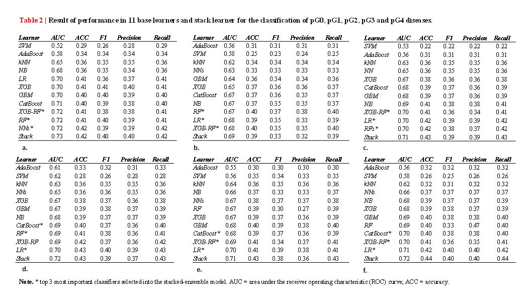
Reducing the feature space dimension aims to select informative characteristics, reduce the risk of bias and potential overfitting. The Pearson product-moment correlation coefficient (PCC) and false-discovery-rate (FDR) U-test was estimated between each pair of features, and random features were removed if the PCC was larger than 0.85 and FDR-test p-value was larger than 0.05. Then the retained features from Radiomics and 5 deep transfer learning embedders were assessed using mean decrease Gini index (MDGI) with a Random Forests (RFs) analysis. MDGI represents the importance of individual features for correctly classifying a residue into linker and non-linker factors. For the prevention of overfitting, only the top-ranked (top 0.1% by MDGI) factors in each imaging profile were selected as the linker factors. Next, the linker features selected from imaging embedders such as Radiomics, DeepLoc, SqueezeNet, Inception v3, VGG16 and VGG19 were integrated into six imaging signatures using multi-class classification with weighted classifier selection and stacked-ensemble learning. The first layer of our stacked ensemble learning framework has 11 base learners including AdaBoost, k-Nearest Neighbors (k-NNs), Support Vector Machine (SVM), Neural Networks (NNs), Naïve Bayes (NB), Logistic Regression (LR), RFs, Gradient Boosting Machine (GBM), Extreme Gradient Boosting (XGB), Extreme Gradient Boosting with Random Forest (XGB-RFs) and CatBoost, whose outputs are concatenated and then fed into the next layer, which itself consists of multiple stacker models. These stackers then act as base models to an additional layer. We performed a random search over the parameter configuration, and chose the optimal parameters with the best score based on the evaluation of log-loss of stacked model on 5-fold cross-validation datasets. The details of hyper-parameter set configurations of 11 base learners are summarized in supplementary data (Table S2). The outputs calculated from the stacked ensemble predictors indicated the relative risk that the patient has pG0, pG1, pG2, pG3 or pG4 diseases. Finally, six imaging embedded signatures, i.e., Rad, TLIS-DeepLoc, TLIS-SqueezeNet, TLIS-Inception v3, TLIS-VGG16 and TLIS-VGG19, were built for characterizing PCa Gleason grade with mpMRI.
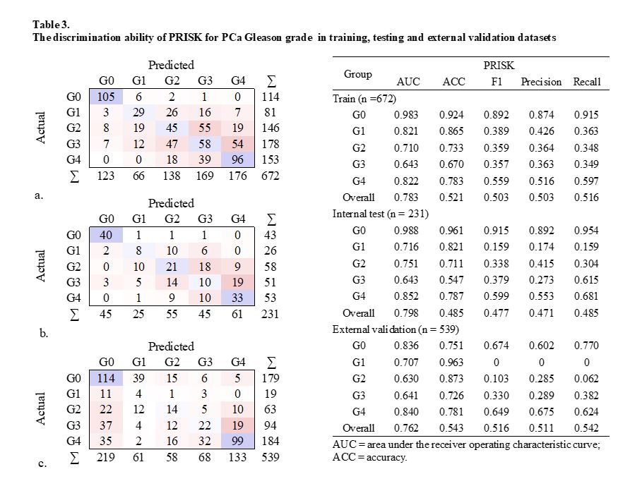
In order to evaluate synergistic effects of multimodal integrations on the prediction of PCa Gleason grade, the 6 newly developed imaging signatures were combined with 4 clinical variables such as patient age (≤ 60 yrs, > 60 yrs), PSA level (4–10 ng/ml, 10–20 ng/ml, 20–100 ng/ml and > 100 ng/ml), location of observation (peripheral zone [PZ], transition zone [TZ]) and a PI-RADS score from radiologists’ reports. An interpretable risk assessment model (PRISK) was developed using a multinomial LR with elastic net penalty. The PRISK model is based on proportionally converting each regression coefficient in multivariate LR to a 0- to 100-point scale. The effect of the variable with the highest β coefficient (absolute value) is assigned 100 points. The points are added across independent variables to derive total points, which are converted to predicted probabilities (Pi). The performance of PRISK model was independently tested on 232 internal test datasets, and on 539 external validation datasets. The entire flowchart of the study design is showed in Fig. 1.
Predictors of prognostic outcome
Additionally, we prospectively evaluated a Cox proportional hazard regression model using 5 clinical and imaging factors including age, PSA, PI-RADS score and a PRISK score to assess the incremental aspect of our PRISK calculator on predicting BCR of PCa after RP in 462 PCa patients who underwent RP treatment.
Statistical Analysis
Quantitative variables were expressed as mean ± standard deviation (mean ± SD) or median and range or median and range, as appropriate. Model performance was typically evaluated against a “ground truth” with imaging-histopathological annotations using receiver operating characteristic (ROC). Detection rates such as true positive, true negative, false positive and false negative rate were reported using a confusion matrix analysis. The Cox model’s performance was evaluated based on Harrell’s concordance index (C-index), calibration curves and Kaplan-Meier survival analysis. All the statistics were two-sided, and a p-value less than 0.05 was considered statistically significant. All statistical analyses were performed using MedCalc software (V.15.2; 2011 MedCalc Software bvba, Mariakerke, Belgium) and R software package (V.4.0.2; https://www.r-project.org).