Study area
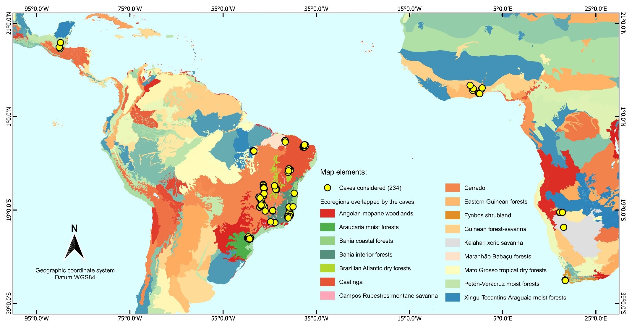
For the survey of biotic and abiotic data, we considered 234 caves in the Afrotropical and Neotropical regions (supplementary material S2), which are found in five countries: South Africa, Brazil, Guatemala, Ghana, and Namibia. These caves are concentrated between 17 ° N and 26 ° S latitudes (supplementary material S1, supplementary Fig. 1) and overlap with 2 biogeographic domains, 3 lithologies, 5 biomes, 16 ecoregions and 26 drainage basins (supplementary material S2).
Biotic data
For the biotic data collection, we first considered the data belonging to the repository from the Center of studies on Subterranean Biology - CEBS, (http://www.biologiasubterranea.com.br/en/) which comprised 191 caves distributed in Brazil, Guatemala and Namibia. Then, we considered data from scientific articles published in peer-reviewed journals, which comprised 43 other caves located in Brazil, South Africa and Ghana62–66. We defined three criteria for the selection of articles used to build the database, which limited considerably the inclusion of caves. Such criteria were: a) Articles in which the emphasis was clearly on surveying fauna or ecological studies involving the entire invertebrate community; b) Articles that provided georeferenced locations of the inventoried caves; c) Articles in which the methodology also indicated active collection (direct intuitive search67), where the collection team searches the entire cave in search of organisms. Having met all the criteria, we used the data on the occurrence of invertebrate families of these caves. The use of family-level was due to two main reasons. First, due to its older origins and distributions generally broader than genera and species, enabling comparisons between areas on a wide geographic scale1,38. Second, we assumed that the sampling and group identification biases have been reduced and homogenized with these measures. Therefore, further taxonomic refinements were avoided. Such refinements have a greater probability of identification errors and uncertainties regarding the distribution of species or genera. These problems have been reported as a major obstacle to studies in invertebrate ecology32,68. The nomenclature of families included in the construction of the database was checked in the literature to verify their current taxonomic situation, where we were able to correct possible synonyms or reclassifications. In this case, just for the construction of the graphs in figure 1, 57 families were assigned to the taxon “Acari”, which is a generic term used to designate six orders of arthropods whose phylogeny is still not well resolved69.
Abiotic data
The abiotic data encompassed information about the surface ecological regions, lithologies, and drainage basins that overlapped the locations of the caves. The delimitations of the ecological regions were obtained from shapefiles with the biogeographical domains, biomes, and ecoregions, on the Ecoregions201733 platform. The delimitations of the drainage basins were obtained from shapefiles on the HydroSHEDS36 platform, where the drainage borders are provided in files with the name “bas” for each continent70. These delimitations indicate divergent drainage flows in the landscape, according to water flow modeling from radar images from the Shuttle Radar Topography Mission (SRTM)36. For contextualization, the definition of the drainage basin we used was that of “a landscape in which the surface waters converge to a single location, such as a point in a stream or river, or a single wetland, lake or other body of water”71.
The locations of the 234 caves were surveyed in the articles considered and into the CEBS database. These locations were then projected in decimal degrees and using the wgs84 datum to meet the specifications of the previously mentioned shapefiles. From the locations, the values for each shapefile were extracted with the Point Sampling Tool from Qgis 3.8.3 software72, and later used in the other steps. The caves, according to information gathered from the CEBS database and from the literature used, belong to carbonate, siliciclastic and granitoid lithologies (Dataset S1).
Statistical procedures
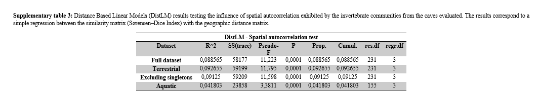
Before testing our hypotheses, we first verified a possible effect of spatial autocorrelation on the similarity patterns of cave fauna, where considerable positive effects are recurrent in this field of study due to the restricted patterns of subterranean fauna dispersion13. For this, we used Distance-based Linear Models (DistLM) to calculate a simple regression73 between the similarity matrix, obtained with the Sørensen–Dice index, and the geographic distance matrix, obtained with the georeferenced locations of the caves. For these cases, these multivariate models are treated as a more robust alternative for the Mantel test73, which is often used to test such influences74. In the regression obtained with the DistLM, the criterion used for the calculation was R²73, with the X and Y coordinates treated as a “geographical distance” indicator and being considered the predictor variable.
Factor testing
The analysis of the factors was carried out systematically, respecting their spatial hierarchy, so that we could filter all possible significant variations within the groups of caves according to the test of each factor.
To form spatial aggregations of caves based on the factors that best represent variations in compositional similarity, we explored five different factors, both separately and combined, with their different number of levels in parentheses (infographic in figure 6): biogeographic domain (2), lithology (3), biome (5), ecoregion (16), and drainage basin (26). We have selected these five factors due to their reported influence on cave communities, where in some ways subterranean communities can be influenced by cave lithology37; by the regional pool of surface species24, an influence that was tested here using the boundaries of the biogeographic domains, biomes, and ecoregions; and finally, by the drainage flows in the landscape, which influence had been only reported acting on strictly aquatic cave organisms until then29,54.
The similarity between cave fauna was obtained using the Sørensen–Dice index, which is less subject to loss of sensitivity in highly heterogeneous datasets75. In addition to being heterogeneous, we found in our data a large asymmetry in the experimental design, where there was a variation in the number of levels of a nested factor within the higher-level factor. For these reasons, we tested significant differences in the faunistic composition of the caves grouped by each factor with the Permutational Multivariate Analysis of Variance (PERMANOVA) in two different designs. PERMANOVA was chosen because it allows testing of the effect of factors by obtaining p-values in highly unbalanced experimental designs, enabling more robust interpretations for these cases73,76.
In the first design, p values were obtained for each factor separately after 9999 permutations with the Type III Partial and Unrestricted Permutation of Raw Data73 criteria. The second design consisted of nesting the five factors hierarchically, with the first factor fixed (biogeographic domain) and the others with their randomized levels (lithology, biome, ecoregion, and drainage basin), obtaining the p-values after 9999 permutations with the Type III Partial and Permutation of Residuals Under Reduced Model73 criteria.
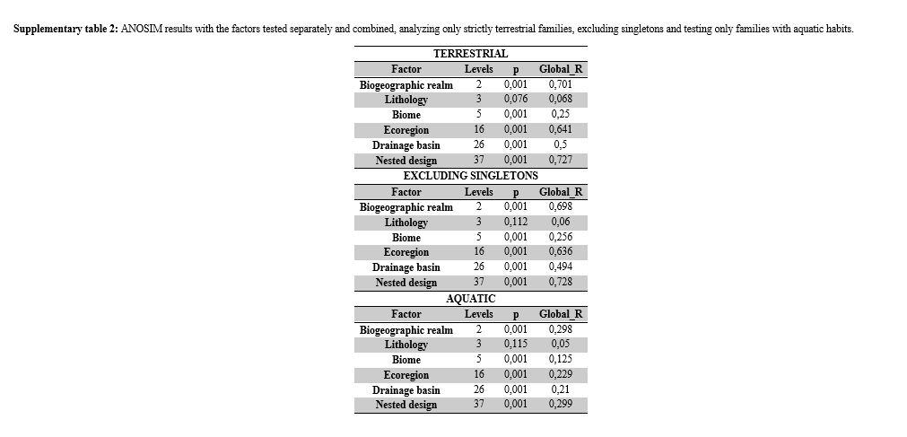
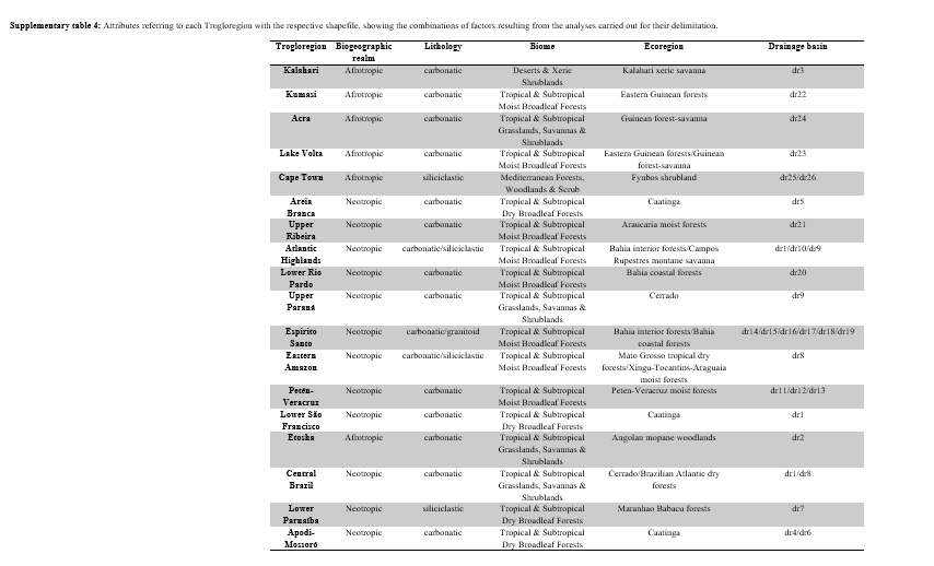
The nested combination of these factors, from the one with the highest number of levels to the one with the lowest number of levels (From “Drainage basin”, with 26 levels, to “biogeographic domain”, with two levels) resulted in the distribution of the 234 caves in 37 groups. Therefore, the caves of each group belong to a combination: drainage basin (Dr) “A”, ecoregion (Ec) “B”, biome (Bi) “C”, lithology (Li) “D” and biogeographic domain (Do) “E” (see the schematic model in figure 7). Despite the low influence shown by the lithology factor in the similarity patterns (PERMANOVA p <0.001, ANOSIM R = 0.063), we opted to maintain this factor in the combination nested with the others tested factors. This standardization of cave groups regarding their lithology is important, as this is a factor that may have a more evident influence on taxonomic categories lower than the level of invertebrate families37.
With the significance assessed, the global R from the Analysis of Similarity (ANOSIM) was used to verify the quality of the cave groups formed according to the factors14, where the higher the global R, the greater the difference between the levels of the factor73. As with PERMANOVA, here we tested the factors separated and combined hierarchically. For ANOSIM, 999 permutations were used.
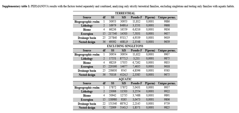
In addition to being applied to the whole biotic dataset, the aforementioned analyses were applied separately only to groups of strictly terrestrial organisms, to aquatic groups (here, we consider as aquatic groups those families with species that need or live associated with water bodies by least at some stage of its life cycle) and excluding singletons from the data. We decided to show only results of the complete dataset in the main text due to its greater robustness since we have found results that showed the same patterns in the other approaches (supplementary material S1, supplementary tables 1, 2 and 3). For these reasons, we carried out the steps described below only for the complete biotic dataset.
For this set, we graphically represented the dissimilarities between the faunistic composition of the caves with the Non-metric Multidimensional Scaling (nMDS), indicating the factors separated and combined hierarchically.
Cave groups delimitation
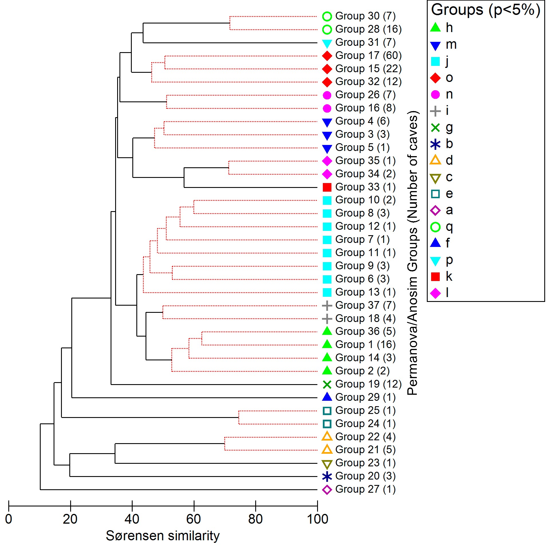
According to the ANOSIM results, the use of the combined factors was selected due to the higher Global R-value. The presence/absence of family data was then computed at the 37 levels resulting from the nested combination of factors, with each level representing a distinct group of caves. These cave groups served as a base spatial unit for the similarity test between the different regions covered, which was carried out through Cluster analysis (CLUSTER) along with Similarity Profile analysis (SIMPROF), both based on the Sørensen–Dice similarity index. The CLUSTER was obtained using the average linkage clustering method, condensing the samples from the closest neighbors by pairwise comparisons77. The SIMPROF analysis added to the CLUSTER is a robust alternative, based on permutations, for the condensation of groups or samples that a priori have an unknown structure based on similarity77. With 999 permutations and testing a significance level of 1% (results in the main text) and 5% (supplementary material S1, supplementary figure 2), respectively, SIMPROF indicated the formation of 17 “supergroups” in which caves have statistically distinct faunistic compositions, thus establishing large regional groups of invertebrate families. Based on these 17 supergroups, we carried out the final Trogloregion delimitation.
Finally, with the 37 initial groups resulting from the nested combination of factors, we calculated another PERMANOVA (9999 permutations, Type III Partial and Unrestricted Permutation of Raw Data criteria) and ANOSIM (999 permutations) using the 17 supergroups indicated with CLUSTER and SIMPROF as the clustering factor. The dissimilarity patterns between these groups were plotted with an nMDS.
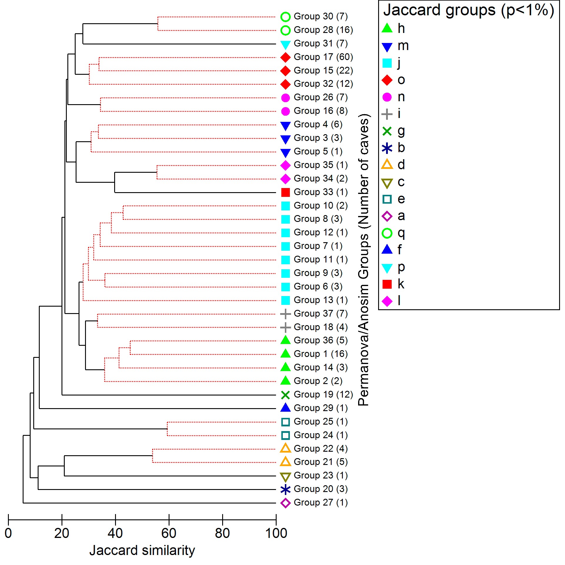
To obtain a counterproof from the supergroups used to delimit the Trogloregions, we calculated another CLUSTER and SIMPROF with 1 and 5% significance levels, this time using the Jaccard index (supplementary material S1, supplementary figures 3 and 4). The Jaccard index maintains the same weight for shared and unique biological groups, resulting in comparatively lower similarity values75. However, these new tests showed us the same supergroups, unchanged. Thus, we have decided to keep the results obtained with the Sørensen–Dice index with p <1%, which presented more robust values, in the main text.
All the above-mentioned analyzes were performed in the PRIMER 6 software with its PERMANOVA + expansion73.
Map construction
Maps delimiting trogloregions were constructed respecting the hierarchical sequence of the five factors used in the other analyzes. Therefore, the initial cutouts (37, according to PERMANOVA and ANOSIM) consisted of the intersections resulting from the vector layers of the ecoregions with the overlapping drainage basins (the ecoregions are already naturally nested in the biomes and biogeographical domains). These outlines were obtained with the Intersection vector tool72. Discontinuities in vector layers without caves were disregarded, and only features with caves were selected. For this, the Multiparts to Single Parts vector tool was used72.
From the outlines, it was possible to carry out the selection and combination of the 37 groups of caves indicated with PERMANOVA and ANOSIM in the 17 supergroups indicated with the CLUSTER and SIMPROF analyses. For the construction of the maps, we split two of the 17 supergroups for having combined caves from different ecoregions and basins which borders are separated by a great geographical distance. Therefore, we split the supergroup that combined caves from the Cerrado ecoregion with caves from the Bahia coastal forests ecoregion (formerly the “i” supergroup, now the “Lower Rio Pardo” and “Upper Paraná” Trogloregions). The other splitted supergroup had combined caves in the Caatinga ecoregion, in the Neotropical region, with caves in the Angolan mopane woodlands ecoregion, in the Afrotropical region (formerly “n” supergroup, now “Kalahari” and “Lower São Francisco” Trogloregions). Four "supergroups" in the CLUSTER/SIMPROF (A, C, F, and K) have only one cave and are considered outliers78, they have very different compositions. This did not allow their combination with the other supergroups according to the analyses. Of these four, the supergroup “k” was combined with “l” because they overlap spatially for sharing attributes (except the lithology, supergroup k has a limestone lithology, while l has siliciclastic lithology), thus forming the “Eastern Amazon” Trogloregion. After these adjustments, the maps indicate 18 Trogloregions, which were named according to some striking geographic feature in their locations.
The shapefile resulting from the maps construction and Trogloregions delimitation contains all information inherent to the factors combined in its attribute table are available as supplementary files (supplementary material S3, and supplementary material S1, supplementary table 4), aiming at its application in future studies and sharing with the scientific community.
The steps described for the construction of the map were performed using Qgis 3.8.372 software.
Data availability
Three supplementary files with additional information for this study are available (https://figshare.com/s/bf641fb4cd64a99f9ae6). Supplementary material S1 contains four supplementary figures and four supplementary tables with further data exploration. Supplementary material S2 contains a .xlsx file with all biotic and abiotic data, and the factors used. Supplementary material S3 contains the Trogloregions shapefile.