Data Source
As one of the largest and most comprehensive national-level population databases in the world,29 the NHI Database contains healthcare records of 30 million residents of Taiwan, including inpatient, outpatient, and pharmacy services.30 The NHI Database is ideal for longitudinal epidemiological investigation because each beneficiary of the NHI has a unique identification number consistent across all datasets, and can be followed through multiple clinical encounters.31 To maximally retain the population heterogeneity to reflect the real-world impact of SES, we selected a random 25% sample from the eligible adult population in 2000 from the NHI Database by random sampling method based on Floyd’s ordered hash table algorithm to ensure an equal probability of the eligible population being selected. We also excluded patients with missing data before 2006 for appropriate censoring and to ensure two-waves worth of longitudinal data at minimum (Figure 1). This study was approved by the Institutional Review Board at the Chang Gung Memorial Hospital.
Overview of Marginal Structural Modeling
Since patients’ socioeconomic status is a time-varying variable, we adopted marginal structural model (MSM) analysis to investigate the causal relationship between patients’ socioeconomic status as defined by income levels and the quality of care received measured by the rate of preventable hospitalization and the Elixhauser Comorbidity Index (ECI). MSM eliminates the confounding bias in estimating this causal relationship, where the other confounding effects vary over time from wave to wave, and these confounders may act as intermediate variables resulting from previous socioeconomic statuses at the same time.37,38 The observational data lack counterfactual outcomes that would have occurred under the opposite exposure level or treatment decision.40 Thus, cross-sectional observational studies use stratification or multivariable regression analyses to address potential confounding and make causal inferences. However, with longitudinal data for which the time-varying confounders (variables that are associated with both treatment and the subsequent outcome) and treatment by indication (variables affected by prior exposure and affect future exposure levels) co-exist, these traditional analyses cannot account for the dynamic effects of the time-varying covariates appropriately to make a causal inference.39 MSM provides an approach to balance out the potential confounding effects in a longitudinal study by creating a pseudo-population to mimic the data from a sequentially-randomized trial, and use that to estimate the average effect of a treatment or an exposure on potential outcomes.41 We chose to use MSM to answer our research question because of these advantages that permit unbiased assessment of the causal effects of SES on the quality of care received in a longitudinal study. We conducted two separate models, each with a different outcome variable: one with the rate of preventable hospitalization and the other with the ECI.
Variables of Interest
We considered preventable hospitalization and comorbidity as representative outcome measures of the quality of care in the community.9 A patient was considered to have had a preventable hospitalization if the primary diagnosis code associated with the inpatient stay was included in the set of diagnosis and procedure codes defined by the Agency for Healthcare Research and Quality for 11 of ambulatory care sensitive conditions32 for which hospitalizations can be avoided with good outpatient care.20,21,33,34 We calculated each patient’s Elixhauser comorbidity index (ECI) 35 by defining it as having ≥2 ambulatory visits or one hospital admission with a corresponding diagnosis code to ensure the validity of indices greater than zero. The first model with preventable hospitalization as outcome included ECI as a covariate, and was calculated as a categorical variable with 3 levels (0, 1-3, and ≥4). In the second model with ECI as outcome, ECI was defined as a continuous variable and calculated at years 2004, 2007, 2010, 2013, and 2016; thus ECI was excluded as a covariate from this model. Demographic and clinical covariates included in the analysis were patients’ sex, age, income level, occupation type, urbanization of area of residence, number of outpatient visits, number of hospital admissions, and the physician density of the area of patients’ residence. Occupation categories defined by the NHI program enrollment protocol30 and income levels in Taiwan dollars were collected directly from the NHI Database and were converted to US dollars by the mean exchange rate during each corresponding calendar year.36 We compared demographic characteristics by income groups for each time wave by analysis of variance test and chi-squared test. In our MSM analysis, values at year 2000 for each independent variable was defined as baseline values. Then, the baseline values were used to calculate the time-varying variables at each wave by taking the average value during each time interval for continuous variables and the mode for categorical variables at each wave and two years before each wave. For example, for the number of outpatient visits variable, the average value between 2001 and 2003 was considered as the number of outpatient visits in 2003. To create income groups at each wave, the average income during the time-period up to each wave-year was used. For example, the average income from 2001 to 2008 was used to define the income level at 2009.
Inverse Probability of Treatment Weights
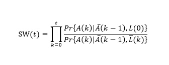
MSM can control the confounding effect of time-dependent confounders without over-adjusting by applying inverse probability of treatment weights (IPTW).42 At each time-point of follow-up, the probability of each patient receiving the treatment/exposure (or not receiving the treatment/exposure, whichever that actually took place) is estimated based on the baseline and time-varying covariates up to that time-point.42 Then, patients are weighted by the inverse of their predicted probabilities of receiving the observed treatment/exposure to create a pseudo-population without the covariate imbalances. Under-represented subjects, given their previous covariate values and treatment history, receive proportionally higher weights, and vice-versa for over-represented subjects. In this pseudo-population, the potential confounders are distributed evenly and thus we can estimate causal effects.39 To reduce the variability and improve the precision of estimation, we applied the stabilized version of IPTW weights42,43 as follows: (see Formula 1 in the Supplementary Files)
Pr{*} denotes the probability function, A(k) represents the time-varying exposure at time k, (k-1) represents the exposure history prior to time (k -1), (k) are the time-dependent covariates through time k that are possible mediators as well as confounders, and L(0) represents the vector of baseline covariates. Here, the numerator contains all covariates measured at baseline, and the denominator contains both baseline and time-varying confounders.42 In our model, weights larger than 50 were considered extreme, and the weights were truncated at 50 in our analysis. To ensure that the confounders were balanced after applying IPTW, we compared absolute standardized mean differences across different exposure groups calculated before and after the weight application.
Censoring/Attrition
To minimize selection bias from inconsistent study cohort at multiple time points, we used censoring weights to account for any loss to follow-up in the data by calculating for the probability of remaining uncensored up to each point of follow-up.44,45 We fit censoring models to predict the probability that a patient remained in the study for each time-interval that the patient actually remained in the study.38 Each subject was weighted by the IPTW multiplied by the inverse probability of censoring weight.42
MSM Analysis
We defined 5 time-waves with 3-year interval between 2000 (baseline) and 2016. The baseline values and time-varying covariates collected up to each wave-year were used to assess their relationships with the outcome variable at each wave-year (Figure 2).
Before applying MSM, we first explored the associations of income quartiles with the outcome and found that outcomes from the higher three income quartiles were very similar. Therefore, we decided to dichotomize the income level into low-income group (<25th percentile) and high-income group (≥25th percentile).
We used a two-stage approach to estimate treatment effects from MSM (Figure 2). During the first stage, we estimated each patient’s probability of being in his or her income group at each time point, and used the inverse of this probability as weights to balance the potential confounding owing to the observed and non-randomized income levels. To acquire the treatment weights (here low-income exposure), we fitted logistic regression models with both baseline variables and time-dependent variables up to each wave (2003, 2006, 2009, 2012, and 2015). Censoring weights were also applied by estimating the survival probability, because the most common reason for discontinuing the NHI coverage was death. Censoring was present at time = t if the patient transferred out prior to or at the next time point t + 1. The final weight for each patient was calculated by multiplying both the treatment weights and censoring weight at each time point. The numerator for treatment weighting was derived by adjusting the baseline values and previous income binary groups in the model and the denominator was derived by adjusting the baseline values and time-dependent variables. The numerator and denominator for censoring weights were obtained from the cox proportional hazard models, with the response variable in cox model as the patients’ binary censoring status.
Then, in the second stage, the causal parameter in the pseudo-population created with each individualized IPTW was recovered by fitting a weighted generalized linear model on the health outcomes (here preventable hospitalization and ECI). We applied IPTW to avoid biased estimation that happens when time-dependent confounders are inappropriately adjusted by stratification or traditional regression approaches. Furthermore, this methodology separates the time-dependent covariates confounder adjustment from the mediation adjustment in assessing the causal impact on the outcome.41,45,46