Study region
Shandong is an eastern coastal province of China and is located between 34° 23′ and 38° 24′ north latitude and between 114° 48′ and 122° 42′ east longitude (Fig. 1). It extends to the Yellow Sea in the east and is bordered by the Hebei, Henan, Anhui and Jiangsu provinces from northwest to southwest. The Shandong province has a total population of approximately 100.47 million and a total land area of 157,100 km2. The gross domestic product (GDP) of Shandong province was 7,646.97 billion Yuan in 2018. Shandong falls in the warm temperate monsoon climate zone, with an annual average temperature and precipitation in the ranges of 11–14 °C and 550–590 mm, respectively. More than 60% of the annual rainfall in the Shandong province is registered in the summer, and high temperatures usually occur in seasons with high precipitation.
Data
From May 1st, 2008 to March 19th, 2009 (47 weeks), weekly HFMD incidence reports for a total of 138 districts in Shandong were collected from the Chinese Centre for Disease Control and Prevention. To reduce the influence of population size, weekly incidence rates were calculated to reflect the risk of the HFMD epidemic for sample locations, and the corresponding Thiessen polygons were constructed to account for spatial effects (Fig. 1). Monthly meteorological data from May 2008 to March 2009 were obtained from the China National Meteorological Information Center (http://data.cma.cn/), including the daily average, maximum, and minimum temperatures (°C), the air pressure (hPa), relative humidity (%), wind speed (m/s), precipitation (mm) and sunshine hours (h). The socioeconomic data were collected from the 2008 statistic Yearbook of Shandong province, including GDP (10,000 Yuan), ratio of the number of primary school students to the total population (%) and number of hospital beds per capita. Spatial Kriging methods were used to calculate the weekly average meteorological factors for each sample location during the 47-week study of HFMD epidemics. Both dynamic meteorological factors and static socioeconomic factors were normalized to the range of 0–1.
Geographically weighted regression model
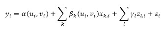
Compared with the global multivariate regression model, local models can be more effective at describing potential local variations in relationships between dependent and independent variables. The geographically weighted regression [33, 34] is a typical local multivariate regression model extensively applied to measure the spatial relationships between variables and corresponding local variations across an entire area. Moreover, GWR model can clearly detect and interpret any non-stationary features of spatial patterns and associations, and has been widely used to estimate the epidemic risk and assess the influence of the epidemic determinants [35, 36]. The GWR model used in this study is as follows:
[Due to technical limitations, this equation is only available as a download in the supplemental files section.] (1)
where yi is the HFMD incidence rate at location i with coordinates ui and vi, α(ui, vi) is the corresponding intercept constant, xk,i are a series of independent variables describing local variations, βk(ui, vi) are the local regression coefficients to be estimated, which vary with location, zl,i are a series of independent variables connected with the global stability, γl are the corresponding stable coefficients, and εi indicates the estimation error.
To approximate the HFMD incidence rate of each sample location in Shandong province, we take the dynamic meteorological factors as the local variables xk in the above GWR model, and the static socioeconomic factors as the global variables zl. Therefore, every location in the study area has a set of specific coefficients to reflect the associations between the HFMD incidence rate and the global or local variables. To solve the proposed GWR model, we apply a Gaussian distance-decay function to represent the relative importance between locations and an adaptive kernel scheme to determine the bandwidth (optimal number of neighboring locations), which is calculated through an iterative optimization process according to the Akaike Information Criterion (AIC). Meanwhile, the significance of the estimated global/local coefficients was checked with pseudo t tests and the model significance was tested by variance analysis (F tests).
Kalman Filter
The Kalman filter (KF) is a data fusion algorithm initially designed to solve the discrete-data linear filtering problem and provides a recursive solution to estimate the state variable of a time-varying system [37, 38]. In this study, KF is used to estimate the HFMD incidence and quantitatively assess the influence of risk factors. For a specific district, we define a multivariate state space X, which includes the HFMD incidence and several static socioeconomic factors. The state space is time-varying and calculated using the following parametric formula:
[Due to technical limitations, this equation is only available as a download in the supplemental files section.] (2)
where Xt is the state vector containing the HFMD incidence and socioeconomic factors at time t, A is the state transition matrix indicating the effects of each state variable at time t-1 on the state vector at time t, Ut is a vector containing control variables which are dynamic meteorological and static socioeconomic factors relevant to this study, B is the control coefficient matrix indicating the effects of each control variable on the state vector, and ωt is a random variable representing the process noise, which is drawn from a zero-mean Gaussian distribution N(0, Q).. Last, Q stands for the prediction noise variance and accounts for the prediction uncertainty compared with the real process. The prediction of the time-varying state vector could be implemented as follows:
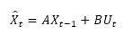
[Due to technical limitations, this equation is only available as a download in the supplemental files section.] (3)
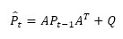
where X̂t is the prediction state vector at time t and Xt-1 is the estimated (filtered) state vector at time t-1. The a priori estimation error covariance of the above prediction model propagates according to the equation:
[Due to technical limitations, this equation is only available as a download in the supplemental files section.] (4)
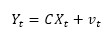
where P̂t is the estimation error covariance of the prediction model at time t. Furthermore, by considering the HFMD incidence Y as the most important variable in the state vector X, we define a simple linear relationship linking the measurement Y to the state vector X:
[Due to technical limitations, this equation is only available as a download in the supplemental files section.] (5)
where Yt is the measurement HFMD incidence at time t which is the observed incidence calculated based on the reported cases, C is the observation operator matrix, and vt is a random variable representing the measurement noise which is also assumed to be drawn from a zero-mean Gaussian distribution N(0, R).. Similarly, R stands for the measurement noise variance and represents the measurement uncertainty.
When both the process prediction and the measurement are considered, the a priori estimation error covariance P̂t and the measurement noise variance R are combined to generate the Kalman gain:
[Due to technical limitations, this equation is only available as a download in the supplemental files section.] (6)
where Kt stands for the Kalman gain at time t and is applied to compute the a posteriori estimation of the state vector at time t as the following linear combination of the a priori estimation X̂t and the actual measurement Yt:
[Due to technical limitations, this equation is only available as a download in the supplemental files section.] (7)
As a function of the state vector covariance and the measurement noise, the Kalman gain Kt is noticeably high if the estimation error covariance is much higher than the measurement noise and the a posteriori estimation of the state vector significantly follows the measurements. Conversely, when Kt is low, the filter will essentially follow the predictions. In fact, Kt establishes the best combination between the process prediction and the measurement in order to minimize the mean square error between the a posteriori estimation Xt and its true value. After the update of the state vector as described above, the a posteriori estimation error covariance can be expressed as:
[Due to technical limitations, this equation is only available as a download in the supplemental files section.] (8)
where I is an identity matrix and Pt indicates the estimation error covariance after the prediction and the update at time t. The a priori estimations take place at each step of the recursive solution based on the last a posteriori estimations, according to Eqs. (3) and (4), the Kalman gain at each step is computed according to Eq. (6), and the a posteriori estimations which are also the a priori estimations of the next step are generated according to Eqs. (7) and (8). Beginning from the initial state, the prediction and the update appear at every single step of the KF recursive solution.
Integration of the Kalman filter with the GWR model
Weekly averages of HFMD incidences in the sample locations were collected; the corresponding spatial autocorrelation was weak, with a Moran’s I of 0.0208 (p = 0.5460). However, the spatial stratified heterogeneity of the HFMD incidence among counties was statistically significant, with a GeoDetector q-statistic of 0.2153 (p<0.001) [39, 40]. Therefore, GWR model was applied to explore the global or local associations between the HFMD incidence and meteorological or socioeconomic factors. The GWR model produced an overall coefficient of determination R2 of 0.2182, which was only an approximately 14% improvement compared with the global regression prediction. These results were possibly caused by the measurement noise in the HFMD incidence, as well as the prediction noise of the GWR model. To better explore the spatiotemporal patterns and assess the determinant factors of the HFMD epidemic, we combined the Kalman filter with the GWR model. The filtering allows to couple the measured and predicted HFMD incidences, and improve the incidence estimation accuracy. On the other hand, GWR model indicates the associations between HFMD incidence and determinant factors, and therefore could provide the prediction modeling of state vector varying in the Kalman filter. Furthermore, the influence sensitivity of the control variables can be evaluated during the incidence filtering process, and the corresponding determinants of HFMD incidence can be quantitively assessed.
In our proposed Kalman filter, the parameter C is a simple observation operator matrix that indicates the transition between the state vector X and the measured HFMD incidence Y. On the other hand, the state transition matrix A models the variation of the state vector that consists of the HFMD incidence and the static socioeconomic factors from time t-1 to time t, while the control coefficient matrix B describes the influence effects of the meteorological and socioeconomic factors on the state vector. Moreover, for different districts in the study area, the global and local effects of the determinant factors on the HFMD incidence vary spatially. Therefore, as shown in Fig. 2, we integrated the GWR model into the Kalman filter, derived the space-varying parameters A and B, and generated multiple filters for the various districts. The HFMD incidence was the explained variable in GWR model, as well as the measurement Y in the Kalman filter. The local and global explanatory variables in the GWR model were the meteorological and socioeconomic factors, which also constitutes the control vector U of the Kalman filter. Moreover, the state vector X in the Kalman filter contains the HFMD incidence and the socioeconomic factors. For each district, the global coefficients γl and the local coefficients βk(ui, vi),, which indicate the associations between the HFMD incidence and determinant factors, were obtained from the GWR result. Thus, the corresponding parameter A in the Kalman filter could be constructed from the global regression coefficients in the GWR model, while the parameter B using the local regression coefficients. Different from the parameters A and C, the control coefficient matrix B is district-dependent (various Bs for districts), and the corresponding multiple filters describe the spatial variation of the HFMD incidence evolution patterns and determinant influence effects.