3.1 Magnetotelluric data
Magnetotellurics (MT) is an electromagnetic method of geophysical exploration used to deduce the electrical resistivity structure of the Earth at depths ranging from tens of meters to hundreds of kilometers. This method uses a source signal of external origin, natural variations of electric and magnetic fields of the Earth, generated by physical processes such as solar variations and magnetic storms. The spectra of these variations cover periods ranging from 10-3 to 105 [s] and are generated by the interaction between the solar wind, the magnetosphere and the ionosphere of planet Earth (Vozoff, 1991).
The MT method is based on the simultaneous measurement of the total electromagnetic field, i.e. the time variation of the magnetic field B(t) and the induced electric field E(t). The electrical properties of the underlying material can be determined from the relationship between the components of the measured variations of electric (E) and magnetic (B) fields, or transfer functions: the horizontal electric (Ex and Ey) and the horizontal magnetic (Bx and By) and vertical (Bz) field components. The transfer functions consist of a complex impedance tensor which relates the measured electric field components to the magnetic field components and a geomagnetic transfer function which is often called a tipper and relates the horizontal magnetic field components to the vertical magnetic field component. In general the resistivity structure of the earth is three-dimensional obtaining a complex impedance tensor of four components, however, if it is a two-dimensional structure where the resistivity does not vary along the geoelectric strike the diagonal components of the tensor are null as long as the coordinate system is parallel to the strike direction. In this case the two surviving tensor components are related to two independent modes, the magnetic transverse (TM) and the electric transverse (TE). Sometimes if the strike preference angle is known, the tensor can be rotated so that the diagonal components are minimized. Generally the elements of the impedance tensor can be plotted as apparent resistivity and phase as a function of period (reciprocal of frequency), these graphs can give us an idea of variations in the average resistivity of the medium that has been measured so that short periods are related to shallow depths and long periods to greater depths. Some components of the measured electric fields can be affected by a phenomenon called Static Shift that is a galvanic distortion effect that locally shifts apparent resistivity sounding curves by a scaling factor that is independent of the frequency, keeping the phases unchanged. This effect is caused by charge accumulation at boundaries of shallow conductive heterogeneities, which disturb the regional electric field locally (Tournerie et al., 2007). On the other hand, the geomagnetic transfer function serves to identify lateral resistivity contrasts and can be represented as arrows or induction vectors, under the convention of Wiese (1962) the vectors point in the opposite direction to the conducting body. When making long period measurements near the ocean it is expected to observe the so-called shore effect on the induction vectors for long periods. Due to the large resistivity contrast between the ocean and the continent the orientation of the vectors over longer periods should be expected to be in the opposite direction and perpendicular to the shore.
In order to obtain a lithospheric model of the electrical resistivity structure of the study area, several field campaigns were carried out between December 2018 and April 2019, where 14 long-period and 10 broadband stations were installed along the profile transverse to the coast (fig1). Three types of instruments were used to carry out the measurements, ADU (Analog/Digital Signal Conditioning Unid) with induction coils MFS-07e and electrodes EFP-06, manufactured by Metronix geophysics; NIMS (Narod Intelligent Magnetotelluric Systems) with Triaxial ring-core magnetometer and OSU Pb-PbCl2 gel-type electrodes; and instruments Lemi417 with non-polarized electrodes Lemi-701 and Flux Gate sensor Lemi-424 manufactured by LEMI LLC. All stations were oriented with a geomagnetic coordinate system. The data processing included the application of filters to the obtained time signals to eliminate noise signals where possible, remote reference application in some cases to improve the data quality of the stations that were measuring simultaneously. The signals obtained with ADU stations were processed with the robust process developed by Egbert & Booker (1986), those obtained from NIMS stations were processed with the code developed by Egbert & Livelybrooks (1996) and the signal obtained with Lemi stations were processed with the robust code developed by Egbert (1997).
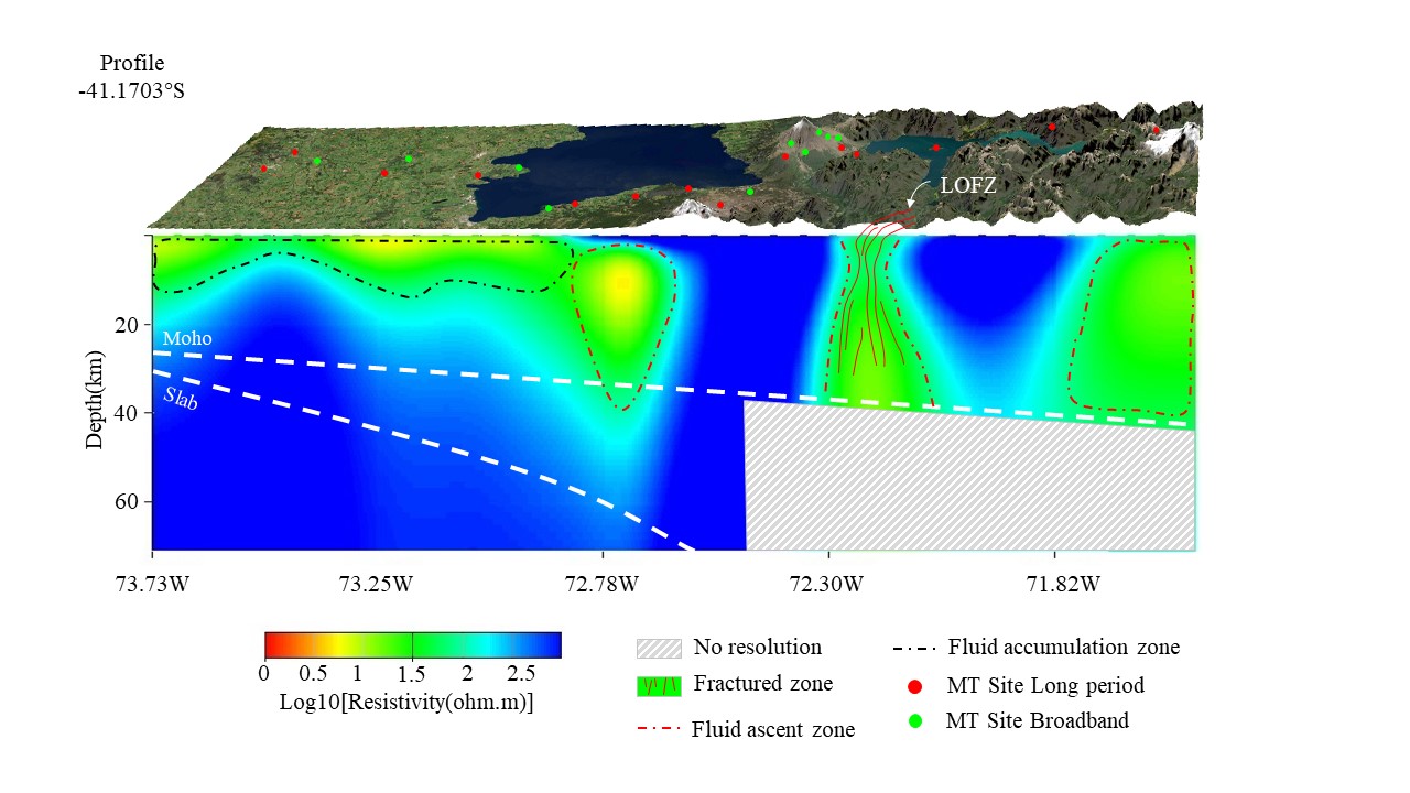
We proceeded to calculate the strike in period intervals for all stations with the code developed by Smith (1995) in order to know if there was any preferential direction of the structure and to diagnose a possible two-dimensional space. In figure 2 it can be seen that for the range of periods between 10-3s and 100s the structure does not have a preferential orientation, evidencing a three-dimensional environment, while for periods greater than 1s the structure begins to behave two-dimensionally. In figure 3 the induction vectors are plotted in a length vs period profile where we can observe characteristic behaviors of areas where we expect to find conductive bodies in the inversion models. The small magnitude of the arrows enclosed by the dotted celestial line and the W-E direction of the arrows enclosed by the purple line suggests a conductive zone towards the west of the Llanquihue lake, the direction of the vectors enclosed by the pink dotted line could be indicating the presence of a conductive body around the Osorno Volcano, while the magnitude of the arrows enclosed by the green dotted line indicates the presence of a body of low resistivity in the Andes mountain range.
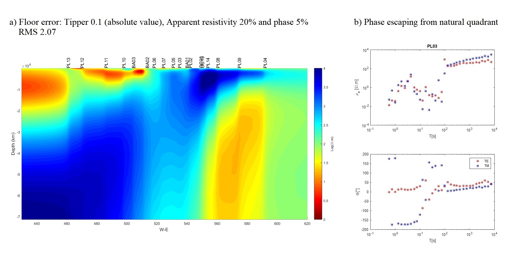
For long periods (>101s), the arrows were expected to have a regional behaviour in W-E direction due to the coast effect, however, it can be observed in the vectors delimited by the yellow dotted line that have a SW-NE direction. This behavior of the vectors is studied by Brasse et al. (2009) in the Chilean continental margin, between latitudes 38°-41°S and they attribute ist to the resultant between the effect of the ocean and the presence of a layer with structural electrical anisotropy in the crust. Anisotropy was also identified in some phase curves that escaped their natural quadrant (see supplementary files). However, phases out of quadrant can also be explained by strong galvanic distortion, 2D structures with high resistivity contrasts, 3D conductive bodies generating strong current channeling or a superposition of different effects (Martí, 2014).
An electrically anisotropic medium can be, for example, a space influenced by micro-scale hydrated faults that can become a macro-scale structure if these structures have a preferential general orientation. From the above, it can be inferred that one way to mitigate the effect of anisotropy on the data is to work with the periods between 101s and 104s, since this range has a general preferential strike (Martí, 2014)
3.2 Magnetotelluric data inversion
We carried out 2D and 3D inversions in order to obtain a realistic model that is close to the geology of the region. In addition, Martí (2014) recommends testing different inversion software, different models and altering different parameters in the inversions until we obtain models without artifacts resulting from structural electrical anisotropy.
For the two-dimensional inversion we used the WinGlink software that uses the 2D inversion code from Rodi & Mackie (2001) , this algorithm minimizes an objective function, by means of the non-linear conjugate gradient method (NLCG), which penalizes the differences between the data and the model response, in order to obtain a contrast of resistivities in a smooth model. Taking into account the dimensional analysis performed previously, the data set was chosen between the range of periods 101s and 104s. The field measurements were made with respect to the magnetic North and the general strike calculated for periods greater than 10s (N8°E) is approximate to the geological structures in the area, so it was decided not to rotate the data since it is assumed that the regional resistivity structure can approximate a 2D structure that varies in the E-W direction, parallel to our profile. As the anisotropy is mostly reflected in the induction vectors, it was chosen to model only the TE and TM mode impedance data.
Background resistivities of 100 and 500 𝛺.m were tested. For longer periods the same result in both tests were performed. The minimum frequency used was 0.00008hz, error floors were set to 20% for apparent resistivities and 5% for phases. A fine grid with growth factor 1.2 was used in depth and to the sides of each station. Although, the topography option was activated, it is not influential in the inversion when working with long period data. Some initial tests were performed varying the regularization factor until a tradeoff between roughness and RMS was found, the value was set to 𝜏 = 8.
To the initial inversion known information of the zone was delivered, an ocean was drawn with a resistivity of 0.3 𝛺m and a mean depth of 5 km according to the bathymetry registered by the National Oceanic and Atmospheric Administration (www.ngdc.noaa.gov/mgg/topo/topo.html).
In order to mitigate the impact of anisotropy on data, separate tests of inversions of the tipper and the TE and TM modes were carried out, following recommendation of Martí (2014), Additionally, a joint inversion of the TE, TM modes and tipper was made assigning a high error floor to the tipper according to Brasse et al., (2009) (see supplementary files). Eventually, a model that does not include the tipper data was chosen, since the same bodies with a lower RMS were obtained. It should be noted that there are other methodologies to identify anisotropy in the data through dimensional analysis (e.g., WALDIM, Marti et al., 2009) near our study area, Kapinos (2011) performs forward methodology to model anisotropic layer that explain the anomalous behavior in the data. Therefore, it is clear that the models presented in this study are not ultimate but working with electrical anisotropy is too complicated and there are no computational tools available at the moment.
From the results of 2D and 3D models of synthetic and real data, Chang-Hong et al. (2011) show that it is possible to interpret 2D profile data using 3D inversion method; Provided that use all components of the impedance tensor, can be obtained not only a reasonable image beneath the profile but also reasonable pictures of nearby 3D structure.
There are several MT studies, which deliver 3D models from data collected along a 2D profile, for example, Meqbel et al. (2016), Patro & Egbert (2011) and Beka et al. (2016).
For the three-dimensional model, a logarithmic grid was designed according to the order of periods and the maximum depth expected to be reached with each set of data. The growth factor in x and y direction was set at 1.3 while 1.2 was chosen for the depth (Kelbert et al., 2014).
A total of 52 frequencies were used for the impedance tensor and 50 frequencies for the tipper. The smoothing factor was set at 0.7, according to Slezak et al. (2019) with small values (0.3, 0.4) the inversion algorithm fits the transfer functions by modifying only the small local surface structures. The error flor was 7% |Zxx Zyy|1/2 and 5% |Zxy Zyx|1/2 and the tipper(Tzx and Tzy) was 0.05 (absolute value), as a result of the better quality of the data present in the components outside the diagonal and the Tipper. For this model the bathymetry of the Pacific Ocean was taken into account, this was downloaded from the National Oceanic and Atmospheric Administration and with an electrical resistivity defined at 0.3𝛺m.
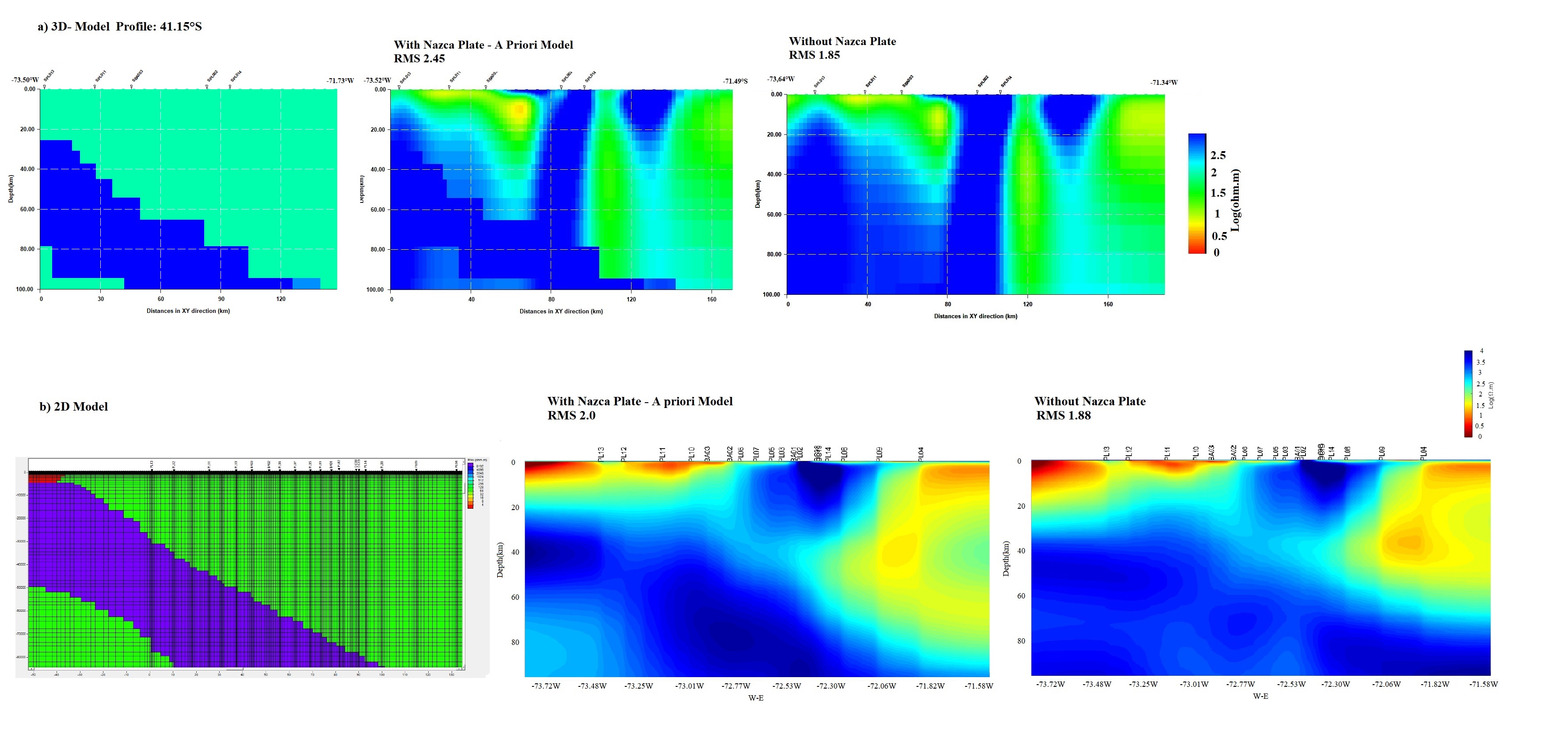
Tests were performed including and excluding the Nazca plate in the 2D and 3D grids of the a priori models (see supplementary files), the Nazca plate was drawn as a layer of 9.000𝛺m taking into account the study of Cordell et al. (2019), resistivity with the depths indicated in the study by Tassara & Echaurren (2012) that presents a model of the depth of the Slab, the continental moho and the contact between lithosphere and asthenosphere in our study zone. We observed that the bodies generated in each case were similar in location, magnitude and shape, however we obtained better RMS in the models that did not include the Nazca plate.
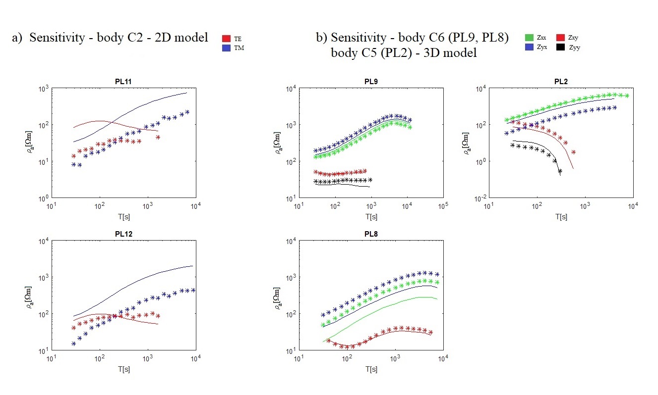
Finally, we performed sensitivity analyses in both models obtained in order to validate the need of each body within the model for the final fit of the curves of each station.
The sensitivity analysis consists of eliminating the structure and studying the response of the model through forward modeling. The response of the new model is compared with the response of the original model to investigate how it is modified when a body is removed. If the variation influences different stations and the size and distance to the location of the body is consistent with the perceived fluctuation in the curves of each site, it can be concluded that the body is necessary for the fit of the observed data (see supplementary files).