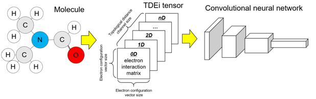
Transformation of molecular structure into tensor shape
In QM calculations, molecular orbitals were calculated through a linear combination of AOs, and coefficients for each AO were estimated during the calculation in the density matrix, which is a diagonal matrix whose rows and columns are all AOs in a molecule. As a molecule can be translated into a matrix format with AO information, the concept was used with adaptations in the TDEi tensor design. First, the Ei matrix was designed with rows and columns with a fixed size of the EC vector such that every input has an identically sized matrix. The size of the density matrix is dependent on the number of AOs in the molecule; however, the input shape must be equal regardless of the size of the molecule in order to input them into the CNN. As the size of the Ei matrix was fixed, molecular geometry differences were lost in the matrix because the EC vector was solely based on the composition of molecules; however, molecules with identical compositions can have different molecular geometries. To consider the difference in the topological structure of a molecule, a matrix was generated based on the topological distance within a molecule.
The matrix for the topological distance 0 is shown in Fig. 2A. Topological distance 0 means the atom itself; thus, the EC vector of a C atom was multiplied by a row and a column in order to calculate the number of interactions between all electrons within the C atom. The topological distance 0 matrix is the sum of the Ei matrices for all atoms within a molecule. The matrix for the topological distance 1D is explained in Fig. 2B. Further, the pairs of atoms within the molecule were considered to calculate the Eis between them. As the Ei matrix was calculated for all atoms in a molecule, the Ei matrices between the C and N atoms were calculated twice in the example. Therefore, they were divided by two, and all Ei matrices for topological distance 1D were added. All Ei matrices with topological distances greater than 1 were calculated, as explained in Fig. 2B. In QM calculations, chemical bond information is not required, thus the physical distance between the atoms was measured based on the coordination of each atom. The precise 3D geometry of a molecule should be prepared to accurately calculate the physical distance between atoms. However, 3D geometry optimization requires an expensive computational cost, and it is not suitably accurate. Hence, 2D structural information alone was used, and the topological distance between atoms was used in the TDEi tensor calculation. The GetDistanceMatrix function implemented in RDKit was used to obtain the topological distance of atoms within a molecule once hydrogen was added to it.
The Ei matrix can be calculated from the topological distance. In the example molecule (Fig. 3), atom pairs existed up to a topological distance of 4D. The Ei matrices from atom pairs with greater topological distance can be calculated if the size of the molecule increases. When Ei matrices were prepared from a range of predetermined topological distances, they were concatenated to form the TDEi tensor (Fig. 4). As the TDEi tensor size can be varied based on the size of the EC vector and the topological distance, it can be flexibly adjusted according to the size of the data or the diversity of chemical space.
Datasets
In this study, four datasets were selected for the regression tasks: melting point (MP), water solubility (Esol), octanol/water distribution coefficient (Lipop), and hydration free energy (Freesolv). There are various publicly available datasets for the classification problem that are used in deep learning model development studies [9, 10, 13, 17] such as human immunodeficiency virus replication inhibition (HIV), human ß-secretase 1 inhibition (BACE), blood-brain barrier penetration (BBBP), toxicity in clinical trials (ClinTox), drug adverse reactions (SIDER), biological targets screened in Tox21 and ToxCast, and PubChem BioAssay data (MUV); however, they were not used in this study because labels in the datasets were seriously imbalanced, whether they were binary, or multiple classification tasks.
MP was obtained from the study by Igor V. Tetko et al., in which 275,131 compounds were extracted using their normal melting point values by mining patent documents [22]. The dataset was divided into training, validation, and external test sets by a random split, in a ratio of 8:1:1. It is the largest publicly available, labeled chemical dataset. ESOL, Freesolv, and Lipop were obtained from the study by Jian et al. [17]. Because the datasets were already divided into the three given categories by the authors, I used them as such. The number of data and the range of the endpoint are listed in Table 1, and the chemical space of the datasets were plotted to verify the structural diversity in the training, validation, and external test sets (Fig. 5).
Table 1
Datasets for model building
|
Endpoints
|
Totalnum.
|
Trainining set
|
Validation set
|
Test set
|
|
Num.
|
Range
|
Num.
|
Range
|
Num.
|
Range
|
|
MP
|
275,131
|
220,104
|
-199.0 to 517.0
|
27,513
|
-157.15 to 420
|
27,514
|
-185.18 to 438.65
|
|
Lipop
|
4,193
|
3,354
|
-1.5 to 4.5
|
420
|
-1.42 to 4.49
|
419
|
-1.17 to 4.5
|
|
Esol
|
1,127
|
901
|
-11.6 to 1.58
|
113
|
-9.16 to 0.94
|
113
|
-8.40 to 1.02
|
|
Freesolv
|
639
|
511
|
-25.47 to 3.16
|
64
|
-9.76 to 3.43
|
64
|
-20.52 to 3.12
|
TDEi parameter search
Because TDEi tensors can have different shapes based on EC vectors and topological distances, experiments were performed to determine which option can provide the best prediction outcome for each dataset. Six different EC vectors and topological distances from zero to four were used in the TDEi tensor calculation. Models were developed with identical hyperparameters, such as Relu for the activation function, RMSprop for the optimizer, and identical CNN architecture. Epoch was applied differently because of differences in the size of data, such as 15 for MP and 100 for other datasets, in this preliminary search.
Model development and validation
CNN was used in this study for model development, through Tensorflow 2 [23], and the network architecture was designed based on VGGNet as a backbone with modifications, such as (1) the size of the initial filter channel was reduced by half from that is 64 to 32, (2) the filter shape was reduced from three by three, to two by two, (3) average pooling was used to minimize information loss, and (4) a convolutional layer was applied once before the pooling layer (Fig. 6). A grid search was performed on the CNN architectures, activation functions, and epoch numbers to obtain the finest hyperparameters for model development. Model training was conducted using the NEURON system of the National Supercomputing Center of South Korea (https://www.ksc.re.kr/eng/resource/neuron).
The prediction accuracy of the model was measured using four metrics: mean absolute error (MAE), normalized mean absolute error (NMAE), R square (R2), and Spearman’s rank correlation coefficient (Sr).

where, ypred is a model’s prediction value, yobs is an observation value, n is the number of compounds,  is the average of observation values, and d is the difference between the ranks of each compound. The prediction model with R2 higher than 0.6, on the external test set, is considered as an accurate model. Even though the model did not achieve R2 > 0.6, it was still able to make an accurate prediction of the target value when NMAE was less than 10%. As the QSAR model was used in the prioritization of compounds, Sr higher than 0.6 implies that the model’s prediction is valid and useful in relative comparison of chemicals, even if NMAE is over 10% [24].
Model analysis
CNN models were developed over four datasets; however, the CNN model developed with MP alone was analyzed because this model was trained with the largest dataset. In the QSAR study, the capacity to separate different molecular structures was the most significant point in the descriptor design to facilitate valid predictions using the descriptor. As the CNN extracted features from the TDEi tensor, the performance of these features in distinguishing compounds along the MP was examined. The final model outputs were extracted from the middle of the CNN before the final prediction value was calculated. Principal component analysis (PCA) was used to project extracted features into 2D space, and extracted feature variation was examined to determine how the model correlates with the extracted features for the prediction of target values.