Sample collection
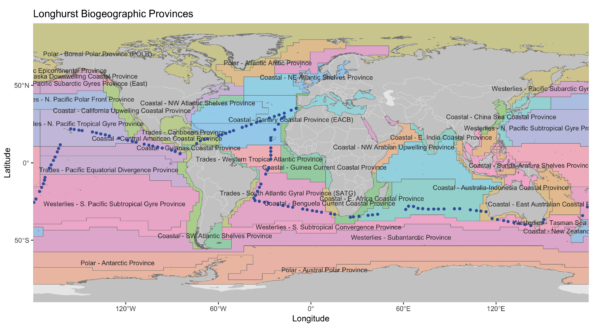
Surface waters (3 m depth) from a total of 120 globally-distributed stations located in the tropical and sub-tropical ocean (Figure 1A) were sampled as part of the Malaspina 2010 expedition [30]. Sampling took place between December 2010 and July 2011 and the cruise was organized in a way so that most regions were sampled during similar meteorological seasons. Samples were obtained with a 20 L Niskin bottle deployed simultaneously to a CTD profiler that measured conductivity, temperature, oxygen, fluorescence and turbidity for each sample. About 12 L of seawater were sequentially filtered through a 20 µm nylon mesh, followed by a 3 µm and 0.2 µm polycarbonate filters of 47 mm diameter (Isopore, Millipore, Burlington, MA, USA). Only the smallest size-fraction (0.2 -3 µm, here called “picoplankton” [8]) was used in downstream analyses. Samples for inorganic nutrients (NO3-, NO2-, PO43-, SiO2) were collected from the Niskin bottles and measured spectrophotometrically using an Alliance Evolution II autoanalyzer (Frépillon, France) [80]. Chlorophyll measurements were obtained from Estrada et al. [81]. In specific samples nutrient concentrations were estimated using the World Ocean Database [82] due to issues with the measurements. Since not all environmental parameters were available for all stations, two contextual datasets were generated: Meta-119, including 119 stations, 5 environmental parameters and 5 spatial features (all except one station in Figure 1A) and Meta-57 (Figure S4, Additional file 7), including 57 stations and 17 environmental parameters (the 5 environmental parameters included in Meta-119 were considered here as well). See Supplementary Methods, Additional file 6.
DNA extraction, sequencing and bioinformatics
DNA was extracted using a standard phenol-chloroform protocol [83]. Both the 18S and 16S rRNA-genes were amplified from the same DNA extracts. The hypervariable V4 region of the 18S rRNA gene (≈380 bp) was amplified with the primers TAReukFWD1 and TAReukREV3 [84], while the hypervariable V4-V5 (≈400bp) region of the 16S rRNA gene was amplified with the primers 515F-Y - 926R [85], which target both Bacteria and Archaea. Amplifications were performed with a Qiagen HotStar Taq master mix (Qiagen Inc., Valencia, CA, USA). Amplicon libraries were then paired-end sequenced on an Illumina (San Diego, CA, USA) MiSeq platform (2x250bp) at the Research and Testing Laboratory facility (http://www.researchandtesting.com/). See additional details on gene amplification and sequencing in Supplementary Methods, Additional file 6.
Reads were processed following and in-house protocol [86]. Briefly, raw reads were corrected using BayesHammer [87] following Schirmer et al. [88] Corrected paired-end reads were subsequently merged with PEAR [89] and sequences longer than 200 bp were quality-checked (maximum expected errors [maxEE] = 0.5) and de-replicated using USEARCH V8.1.1756 [90]. Operational Taxonomic Units (OTUs) were delineated at 99% similarity using UPARSE V8.1.1756 [91], producing 42,505 picoeukaryotic and 10,158 prokaryotic OTUs-99%. Taxonomic assignment of OTUs-99% was generated by BLASTing OTU-representative sequences against different reference databases. BLAST hits were filtered prior to taxonomy assignment using an in-house python script, considering a percentage of identity >90%, a coverage >70%, a minimum alignment length of 200 bp and an e-value < 0.00001. Metazoan, Streptophyta, nucleomorphs, Chloroplast and mitochondrial OTUs were removed from the OTUs-99% tables. See Supplementary Methods, Additional file 6 and Table S8, Additional file 18.
Additionally, to investigate the effects of clustering on the estimation of ecological mechanisms (Fig. 1B), we determined OTUs as Amplicon Sequence Variants (ASVs) using DADA2 [92]. For the 18S, we trimmed the forward reads at 240 bp and the reverse reads at 180 bp, while for the 16S, forward reads were trimmed at 220 bp and reverse reads at 200 bp. Then, for the 18S, the maximum number of expected errors (maxEE) was set to 7 and 8 for the forward and reverse reads respectively, while for the 16S, the maxEE was set to 2 for the forward reads and to 4 for the reverse reads. Error rates were estimated with DADA2 for both the 18S and 16S and used to delineate OTUs-ASVs (see additional details in Supplementary Methods, Additional file 6). A total of 21,970 and 6,196 OTUs-ASVs were delineated for the 18S and 16S respectively.
OTUs-ASVs were assigned taxonomy using the naïve Bayesian classifier method [93] together with the SILVA version 132 [94] database as implemented in DADA2. Eukaryotic OTUs-ASVs were also BLASTed [95] against the Protist Ribosomal Reference database (PR2, version 4.11.1; [96]). Streptophyta, Metazoa, nucleomorphs, chloroplasts and mitochondria were removed from OTUs-ASVs tables. Tables of OTUs-ASVs were rarefied to 20,000 reads per sample with the function rrarefy in Vegan. Only OTUs-ASVs with abundances >100 reads were used for the calculation of ecological mechanisms (Fig. 1B).
We tested the similarity of OTUs-99% and OTUs-ASVs between themselves as well as against a reference database (SILVA v132) in order to determine whether there were differences in the OTUs delineated by UPARSE or DADA2. Comparisons were run using BLAST, and only best hits featuring a sequence similarity >90%, e-value < 0.001, query coverage > 60% and alignment length >200 bp were considered. For the 16S, OTUs-ASVs vs. OTUs-99% displayed a 99.0% (SD=2.0%) mean similarity, while for the 18S both types of OTUs had 99.3% (SD=1.4%) mean similarity. Furthermore, for the 16S, the mean similarity to SILVA reference sequences was 98.8% (SD=1.5%) for OTUs-99% and 98.5% (SD=2.2%) for OTUs-ASVs. In turn, for the 18S, the mean similarity against SILVA v132 was 97.8% (SD=2.0%) for OTUs-99% and 97.2 % (SD=2.5%) for OTUs-ASVs. In sum, these analyses indicate a high similarity between OTUs-ASVs and OTUs-99%, both having also comparable levels of similarity to reference sequences, which indicates that the two approaches to delineate OTUs (i.e. UPARSE vs. DADA2) have similar error-rates.
We used publicly-available data from the TARA Oceans global expedition [31] in multiple analyses. This expedition took place between September 2009 - March 2012, and includes samples from the same hemisphere during different meteorological seasons. Due to the nature of the TARA Oceans dataset, we did not perform all the analyses that were run for the Malaspina dataset. Specifically, short V9 18S rRNA-gene reads or 16S rRNA-gene miTags [97] from TARA Oceans precluded robust phylogenetic reconstructions, which instead were possible with the longer reads produced for Malaspina. We used data from TARA Oceans surface (≈5 m depth) stations only, including 41 samples (40 stations) for pico-nano eukaryotes (0.22-3 mm [1 sample] and 0.8-5 mm [40 samples]; 18S-V9 rRNA gene amplicon data) [34] as well as 63 stations for prokaryotes (picoplankton, 0.22-3 mm [45 samples] and 0.22-1.6 mm [18 samples]; 16S rRNA genes, miTags) [56].
General analyses and phylogenetic inferences
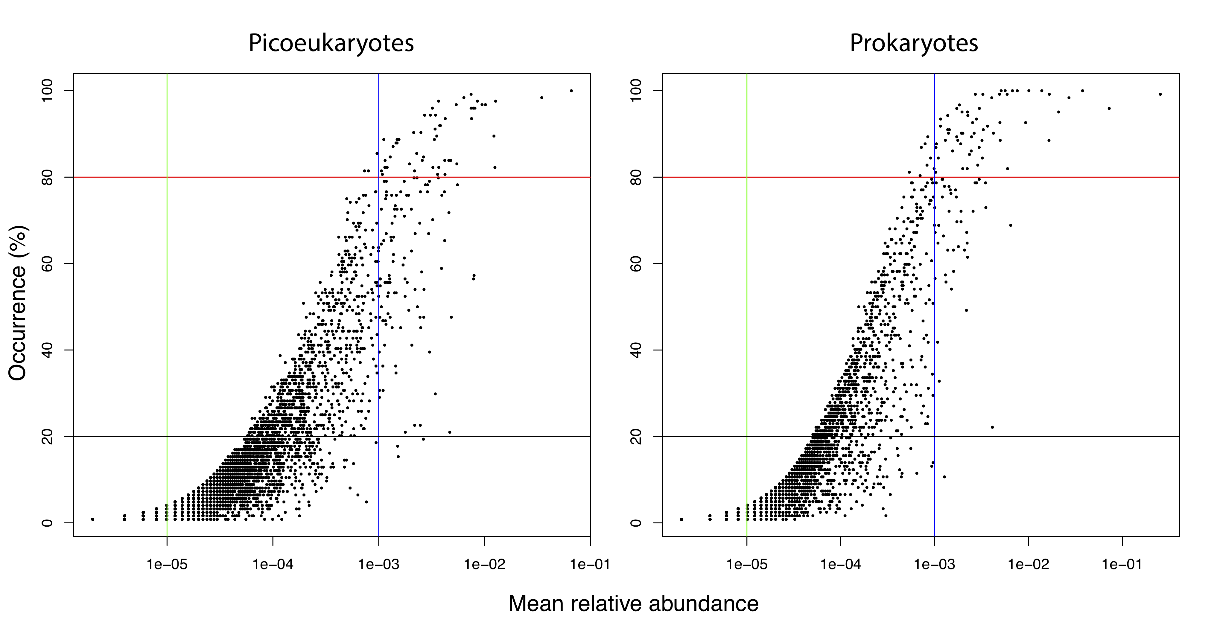
Tables including OTUs-99% were sub-sampled to 4,060 reads per sample using rrarefy in Vegan [98], resulting in sub-sampled tables containing 18,775 picoeukaryotic and 7,025 prokaryotic OTUs. OTUs-99% with mean relative abundances >0.1% or <0.001% were defined as regionally abundant or rare respectively [99]. Phylogenetic trees were constructed by aligning 16S or 18S OTUs-99% representative sequences or OTUs-ASVs against an aligned SILVA [94] template using mothur [100]. Afterwards, poorly aligned regions or sequences were removed using trimAl [101]. Phylogenetic trees were inferred using FastTree v2.1.9 [102]. Most analyses were performed in the R statistical environment [103] using APE [104], ggplot2 [105], gUniFrac [106], Maps, Mapplots, Picante [107] and Vegan. The Vegan function adonis and adonis2 were used to investigate the amount of variance in community composition explained by environmental or geographic variables. Variance partitioning analyses were run with varpart in Vegan and tested for significance with ANOVA. Distance decay, which refers to the decrease in microbial community similarity as geographic distance between communities increases was investigated in R using Mantel correlograms between geographic distance and b-diversity, considering distance classes of 1,000 km. Local Contributions to Beta Diversity (LCBD) [38], which indicates the degree of uniqueness of each community in terms of its species composition, was measured with adespatial [108]. See Supplementary Methods, Additional file 6.
Quantification of selection, dispersal and drift
These processes were quantified using an approach that relies on null models, consisting of two main sequential steps: the first uses OTU phylogenetic turnover to infer the action of selection and the second uses OTU compositional turnover to infer the action of dispersal and drift [23]. The action of selection, dispersal and drift was quantified using both OTUs-99% and OTUs-ASVs. In order to determine the action of selection using phylogenetic turnover, we first checked whether habitat preferences of phylogenetically closely related taxa (according to the 16S and 18S rRNA-genes) were more similar to each other than to those of more distantly related taxa, what is known as phylogenetic signal [109, 110]. We tested for phylogenetic signal using temperature and fluorescence, which were the two variables that explained the highest fraction of community variance. We detected phylogenetic signal at relatively short phylogenetic distances (Figure S10, Additional file 19; Figure S11, Additional file 20), which is coherent with previous work [23, 111, 112]. We measured phylogenetic turnover using the abundance-weighted b-Mean Nearest Taxon Distance (bMNTD) metric [19, 23], which quantifies the mean phylogenetic distances between the evolutionary-closest OTUs in two communities. bMNTD values can be larger, smaller or equal to the values expected when selection is not affecting community turnover (that is, expected by chance). bMNTD values higher than expected by chance indicate that communities experience heterogeneous selection [19]. In contrast, bMNTD values which are lower than expected by chance indicate that communities experience homogeneous selection. Null models included 999 randomizations [23]. Differences between the observed bMNTD and the mean of the null distribution are denoted as b-Nearest Taxon Index (bNTI), with |bNTI|>2 being considered as significant departures from random phylogenetic turnover, pointing to the action of selection.
The second step uses OTU turnover to calculate whether the b-diversity of communities not structured by selection could be generated by drift (i.e. chance) or dispersal. We calculated the Raup-Crick metric [113] using Bray-Curtis dissimilarities (hereafter RCbray) [23]. RCbray compares the measured b-diversity against the b-diversity that would be obtained under random community assembly (drift); randomizations were run 9,999 times. RCbray values between -0.95 and +0.95 point to a community assembly governed by drift. On the contrary, RCbray values >+0.95 or <-0.95 indicate that community turnover is driven by dispersal limitation or homogenizing dispersal respectively [113]. See Supplementary Methods, Additional file 6.
Estimation of interaction-adjusted indices
Taxa INteraction-Adjusted (TINA) and Phylogenetic INteraction Adjusted (PINA) indices were estimated following Schmidt et al. [26]. TINA is based on taxa co-occurrences while PINA considers phylogenetic similarities. TINA quantifies b-diversity as the average association strength between all taxa in different samples. Thus, communities which are identical or include taxa that are perfectly associated will give a TINA value of 1. TINA values will approach 0.5 in communities sharing no taxa or having neutral associations, and approach 0 if taxa display high avoidance. Dissimilarity matrices were generated as 1-TINA and used in downstream analyses (e.g. Figure 3). Full picoeukaryotic and prokaryotic subsampled OTU-99% tables were used to calculate the abundance-weighted TINAw and PINAw. TINAw was calculated using picoeukaryotic and prokaryotic data from 119 Malaspina surface stations (most stations in Figure 1A). In addition, TINAw was calculated using data from TARA Oceans, including 63 surface stations for prokaryotes and 40 surface station for small unicellular eukaryotes (Figure 3).
Associations between taxa and environmental parameters
We analysed whether OTUs-99% displayed associations with environmental variables and between themselves. Firstly, we used the Maximal Information Coefficient (MIC), which captures diverse relationships between two pairs of variables [114]. The Malaspina dataset consisted of 119 stations and 17 environmental variables. In the TARA Oceans dataset, prokaryotes were analysed across 63 surface stations (including 8 environmental variables), while microbial eukaryotes were analysed across 40 surface stations (including 6 environmental variables) [see Supplementary Methods, Additional file 6]. In both datasets, MIC analyses were run using CV=0.5, B=0.6, and statistically significant relationships with MIC ≥0.4 (Malaspina) or MIC ≥0.5 (TARA Oceans) were considered (MIC thresholds were adjusted to the characteristics of the datasets). MIC significance was assessed using precomputed p-values [114]. Secondly, we constructed association networks with the Malaspina dataset considering OTUs-99% with >100 reads using SparCC [115] as implemented in FastSpar [116]. To determine correlations, FastSpar was run with 1,000 iterations, including 1,000 bootstraps to infer p-values. We used OTUs-99% associations with absolute correlation scores >0.3 and p-value<0.01. Networks were visualized and analysed with Cytoscape [117] and igraph [118].