As impacted by strong intense human activity disturbance, the landscape pattern change significantly affects the habitat quality and ecological risk level in the coastal regions. Though numerous researches were conducted in coastal habitat quality and ecological risk, the correlations of habitat quality and ecological risk with landscape metrics in coastal regions have been rarely reported. A scientific question should be addressed is the scientific basis for the sustainable development of coastal regions. Accordingly, Xinggang town, a coastal region in southern China, was selected as a typical coastal region disturbed by robust human activities. Given high-precision remote sensing data, the temporal-spatial variations of habitat quality and ecological risk in the coastal region were analyzed by adopting the methods of InVEST model and ecological risk index, and the correlations of habitat quality and ecological risk with landscape metrics were examined. As indicated from the results, the deterioration of habitat quality and the increase in ecological risk in the coastal region under the disturbance of human activities exhibited obvious distance gradients. The gradient area close to the coastline was the area with the prominent variations of habitat quality and ecological risk. Most landscape metrics were positively correlated with habitat quality and ecological risk, and the correlations were different in a range of distance gradients. Under the rapid urbanization in the coastal region, the rapid expansion of built-up land and the decrease of natural landscapes significantly impacted the landscape pattern index and then altered the habitat quality and ecological risk level.
Research
Variations of Habitat Quality and Ecological Risk and Their Correlations With Landscape Metrics in a Robust Human Disturbed Coastal Region
https://doi.org/10.21203/rs.3.rs-861058/v1
This work is licensed under a CC BY 4.0 License
Version 1
posted
You are reading this latest preprint version
Habitat quality
Ecological risk
Landscape metrics
Spatial-temporal change
Distance gradient
Coastal region
Over the past decades, the coastal landscape pattern has been noticeably altered under the strong interference of human activities, which reveals that the material and energy flows of the ecosystem has been severely disturbed and destroyed (Zhang et al., 2020a; Tian et al., 2021). Landscape fragmentation and complex landscape structure attributed to huge human disturbance will destroy habitat quality and increase ecological risk, which has raised a key problem faced by coastal regions with robust human activities (Zhang et al., 2020b; Zhang et al., 2020c). The analysis of habitat quality and ecological risk are of great significance for promoting sustainable development of social economy, rational use of land resources and ecological planning in coastal regions (Krebs et al., 2014; Paterson et al., 2019; Zhai et al., 2020).
Currently, several studies on coastal habitat quality and ecological risk have been conducted globally. Habitat quality and ecological risks have been assessed in different coastal regions worldwide (Yu et al., 2015; Guan et al., 2017; Abreu et al., 2021; Ding et al., 2021). The assessment of habitat quality placed major stress on single species (Meng et al., 2004) and biological communities (Landry and Golden, 2019). The methods of field sampling, landscape ecology and ecological model have been extensively employed for habitat quality assessment. For instance, habitat quality of juvenile halibut was assessed in the southeastern Bering Sea based on trawl sampling and benthic sampling (Yeung and Yang, 2018). Two different index systems were adopted to assess the quality of benthic habitats in the adjacent waters of Xiaoqing River in Laizhou Bay (Luo et al., 2016). The Integrated Valuation of Ecosystem Services and Tradeoffs (InVEST) model was employed to assess the habitat quality in the coastal regions of the Yellow River Delta in China (Ding et al., 2021). The research scope of ecological risk assessment was developed from the micro assessment at population and community levels to the macro assessment at landscape and regional levels (Landis, 2004; Li et al., 2017; Liu et al., 2018). The assessment methods of ecological risk consisted of multi-index method and landscape ecology method. For instance, Hua et al. (2018) employed the landscape metrics to assess the landscape ecological risk of Xiamen in coastal China. Li et al. (2020) evaluated the ecological risk of heavy metals in soils of Hangzhou Bay, China by the method of the potential ecological risk index.
Furthermore, the factors of habitat quality and ecological risk have aroused the attention of global scholars. As indicated from existing studies, the development of coastal cities reduced the quality of plankton habitat in urban rivers (Krebs et al., 2014). The increase in cultivated land, aquaculture land and industrial land, and the decrease of wetland area and unused land resulted in the significant decline of habitat quality in coastal regions (Zhang et al., 2020c). Beach restoration improved the habitat quality of horseshoe crabs and shorebirds (Smith et al., 2020). River diversion essentially impacted oyster habitat quality in coastal regions of the Mississippi River Basin (Soniat et al., 2013). The increase in built-up and farmland and the decrease in natural grassland and forest elevated the level of ecological risk (Omar and Cabral, 2020). The expansion of urbanization in coastal regions caused an increase of the area of high ecological risk regions (Zhou et al., 2014).
China is known as one of the nations with a long coastline worldwide. China's coastal regions are populated areas and key economic development zones due to location advantage, resource endowment, topography and history. Coastal regions only take up 14% of China's total land area, whereas they contain over 42% of the country's population and more than 60% of total Gross Domestic Product (Cai et al., 2020). Over the past few years, rapid economic development and population growth have led to the deterioration of ecological conditions in China's coastal regions, which have seriously threatened the sustainable development of coastal regions (Meng et al., 2018). Though habitat quality and ecological risk have been assessed in coastal regions of China (Li et al., 2017; Ding et al., 2021), there are few studies on small-scale coastal regions strongly disturbed by human activity in China. In addition, landscape pattern is a key factor of the ecological environment of coastal regions. The correlation of habitat quality and ecological risk with landscape pattern metrics remains unclear.
Accordingly, this study took Xinggang Town, Guangxi Province, south China as an example to analyze the spatial-temporal variations of habitat quality and ecological risk and their correlations with landscape metrics in a robust human disturbed coastal region. The following hypotheses are proposed: (1) Spatial-temporal variations of habitat quality and ecological risk in the coastal region are characterized by distance gradients (from coastline to inland). (2) There are differences in the spatial-temporal change characteristics between habitat quality and ecological risk in the coastal region. (3) Habitat quality and ecological risk are correlated with landscape metrics in coastal regions, and the correlations are different in different distance gradients.
2.1. Study area
Xinggang town is located in the south of Guangxi Province of south China, covering an area of 123.42 km2. This town acts as a critical zone for the development in the Beibu Gulf of Guangxi Province for its favorable conditions (e.g., the natural harbor (31 km coastline), climate and topography) (Fig. 1). The altitude of this town ranges between 0 and 18 m with a flat terrain. It is recognized as a subtropical monsoon climate area with an average annual temperature of 22.6℃ and an average annual rainfall of 1,663.7 mm. As a key agricultural production region, rice and vegetables are broadly cultivated as agricultural crops. Furthermore, there are abundant shallow beach resources and diverse aquatic products. Over the past few years, Xinggang Town has witnessed the rapid economic development and the rapid population growth, and the total population reached up to 65,000 by 2019.
2.2 Data source and processing
In the present study, the remote sensing images (1 m spatial resolution) of Pleiades satellite in 2005 and 2020 presented by Europe Astrium company acted as the data source. With the support of ERDAS software, the following steps of geometric correction, image registration, image mosaic were processed based on 1: 10000 topographic map and field survey. Given the characteristics of the study area, the landscape types fell to eight types (i.e., farmland, aquaculture land, forest, built-up land, road, water body, mudflat and unused land) by using the method of manual visual interpretation. After the field correction, the Kappa coefficient of landscape type data exceeded 0.9, which revealed that it could comply with the data accuracy requirements of the study. By complying with the scope of the study area, Xinggang town fell to gradient Ⅰ (0-2 km), gradient Ⅱ (2-4 km), gradient Ⅲ (4-6 km) and gradient Ⅳ (>6 km) with an interval of 2 km from the coastline to the inland (Fig. 2).
2.3 Methods
2.3.1 Habitat quality assessment method
Landscape type data were adopted to assess regional habitat quality based on the impact intensity, distance and sensitivity of various threat factors in the habitat quality module of InVEST model (Aneseyee et al., 2020; Yohannes et al., 2021). The operation of the module required the data of the habitat type, the intensity and distance of the effect of the threat factors on each habitat, and the sensitivity of the respective habitat to threat factors. The farmland, aquaculture land, built-up land and road obtained from remote sensing interpretation were considered the landscape types significantly disturbed by human, and they were identified as the threat factors. The sensitivity of the threat factors to habitat, the distance and weight of the effect of the threat factors and other parameters were determined based on the expert score, the recommended value of the model user’s guide (Sharp et al., 2014) and related literatures (Han and Dong, 2017; Xu et al., 2019). The parameter settings of habitat quality module are listed in Tables 1 and 2.

Where Qxj denotes the habitat quality; Hj expresses the habitat suitability index; Dxj is the habitat degradation degree; Z equals 2.5, k equals half of the grid cell resolution; Wr represents the weight of the threat factors; ry is the number of ecological threat factors; irxy is the effect of threat factor r in grid y on grid x; βx is the degree of protection (unconsidered in this study); Sjr expresses the sensitivity of the threat factors to different habitats. The assessment results ranged from 0 to 1. The closer to one, the higher the habitat quality would be, while the closer to zero, the lower the habitat quality would be.
2.3.2 Ecological risk assessment methods
From the perspective of landscape structure of regional ecosystem, ecological risk at the landscape level was assessed with the area proportion of the respective landscape component, landscape structure index and landscape fragility index (Wang et al., 2020; Xie et al., 2021).

Where ERIk denotes the ecological risk index of the k fishnet; Aki is all landscape areas of fishnet; Ak is the area of the k fishnet; m expresses the number of landscape types in fishnet; LLi is landscape ecological loss index; Ui represents landscape disturbance index; Ci denotes landscape fragmentation degree; Fi is landscape separation degree; Di is landscape dominance degree; a, b and c respectively denote the weight of fragmentation degree, separation degree and dominance degree, and 0.3, 0.2 and 0.5 are assigned to the values of a, b and c, respectively; Si is the vulnerability index of landscape. Given the ability of each landscape type to resist external influences, the vulnerability index of the respective landscape was assigned as water body =7, mudflat =6, aquaculture land =5, farmland =4, unused land =3, forest =2, built-up land and road =1. The calculation of ecological risk complied with 400 m×400 m fishnets in the study area, and the fishnet tool of ArcGIS software was adopted to generate 847 fishnets in the study area.
2.3.3 Landscape metrics selection
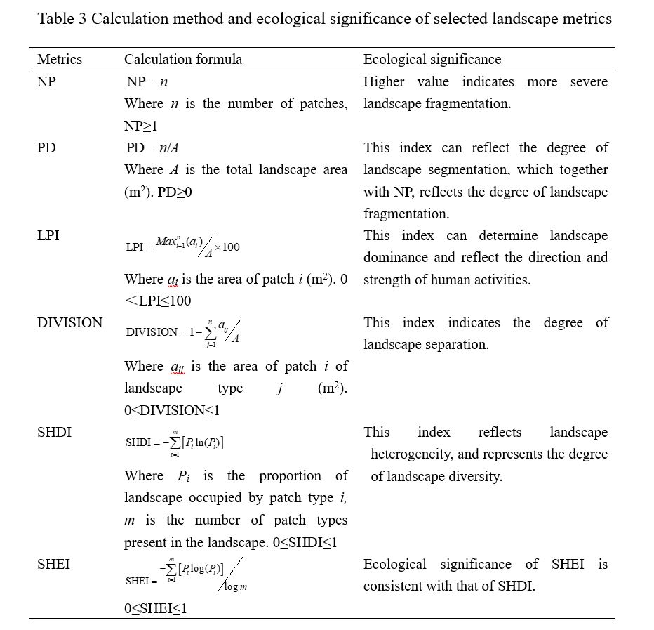
Landscape metrics act as the indicators to quantify landscape pattern, which are capable of indicating the effect of human activities on landscape pattern (Mayer et al., 2016). Six landscape metrics at a landscape level, i.e., number of patches (NP), patch density (PD), largest patch index (LPI), landscape division index (DIVISION), shannon's diversity index (SHDI) and shannon's evenness index (SHEI), were selected to express the landscape pattern in this study (Table 3).
2.3.4 Correlation analysis of landscape metrics with habitat quality and ecological risk
Six landscape metrics (i.e., NP, PD, LPI, DIVISION, SHDI and SHEI) were selected, and the pre-processed landscape type data in 2005 and 2020 were inputted into the Fragstats 4.2 software as the data sources to generate landscape metrics in the respective fishnet. Subsequently, the landscape metrics distribution maps in 2005 and 2020 were drawn with the ArcGIS software. Lastly, the spatial analyst tools of ArcGIS software were employed to generate the spatial map of landscape metrics change in the respective fishnet from 2005 to 2020.
Based on the value of landscape metrics, habitat quality and ecological risk in the respective fishnet, the conversion tool of ArcGIS software was adopted to convert raster data into ASCII files. Next, the correlations of landscape metrics with habitat quality and ecological risk were analyzed by conducting the Pearson correlation analysis in SPSS software.
The Bivariate Local Moran's I tool of GeoDA software was applied for analyzing the spatial correlation of landscape metrics with habitat quality and ecological risk in the respective fishnet, and LISA cluster maps between landscape metrics and habitat quality and between landscape metrics and ecological risk were obtained (Anselin and Sergio, 2014).
3.1 Spatial-temporal change of habitat quality
In the whole region and the respective distance gradient, the level of habitat quality was high in 2005 and low in 2020. Over the past 15 years (from 2005 to 2020), the habitat quality tended to decrease, and the decline of habitat quality decreased with the increase in the distance from coastline (from gradient Ⅰ to gradient Ⅳ) (Table 4).
In 2005 and 2020, the habitat quality in most areas of the study area was low, the area with the habitat quality less than 0.1 dominated the study area, while the area exhibiting the habitat quality of over 0.3 was largely concentrated in gradient Ⅰ. The habitat quality in most areas of the study area tended to decline, and the value of habitat quality decline in most areas ranged from − 0.25 to 0 from 2005 to 2020. The high value (between − 1 and − 0.5) of habitat quality decline was concentrated in the southern part of gradient Ⅰ. Only scattered areas of the town showed the improved habitat quality (Fig. 3).
3.2 Spatial-temporal change of ecological risk
In the whole region and the respective distance gradient, the ecological risk level in 2005 was lower than 2020. The ecological risk tended to increase from 2005 to 2020. The increasing amounts of ecological risk in gradients Ⅰ and Ⅱ were significantly higher than gradients Ⅲ and Ⅳ (Table 5).
In 2005, the high value areas (greater than 1.2) of ecological risk in the study area were concentrated in the central and northern parts of gradient Ⅰ, while the low value areas (less than 0.8) were primarily located in most areas in gradients Ⅲ and Ⅳ as well as the southern part of gradient Ⅰ. In 2020, the high value areas (greater than 1.2) of ecological risk concentrated in most areas in gradients Ⅰ and Ⅱ. The ecological risk values of gradients Ⅲ and Ⅳ were low, ranging from 0.8 to 1.0. The ecological risk in most study area tended to increase except for a small part of northwest between 2005 and 2020. The high value area of ecological risk increase (greater than 0.6) was located in the south part of gradient Ⅰ, and the moderate (between 0.3 and 0.6) was concentrated in the south and east parts of gradient I and the central part of gradient II. The increasing value of ecological risk in most study area ranged from 0 to 0.3 (Fig. 4).
3.3 Landscape metrics variations
The values of other landscape metrics in the whole region in 2020 exceeded those in 2005 except for LPI. The values of NP, PD, DIVISION, SHDI and SHEI in the gradients Ⅰ and Ⅱ exceeded those of the gradients Ⅲ and Ⅳ in 2005, whereas the opposite characteristics were presented in 2020. The value of LPI in gradients Ⅲ and Ⅳ significantly exceeded those of gradients Ⅰ and Ⅱ in 2005, whereas the LPI value in gradients Ⅲ and Ⅳ were lower than those of gradients Ⅰ and Ⅱ in 2020 (Table 6).
Except for LPI, other landscape metrics tended to increase in the whole region between 2005 and 2020. The values of NP, PD, DIVISION, SHDI and SHEI tended to decrease in gradients Ⅰ and Ⅱ, whereas the values tended to increase in gradients Ⅲ and Ⅳ. The trend of LPI in the respective gradient was opposed to that of other landscape metrics (Table 7).
The high values of NP, PD, DIVISION, SHDI, and SHEI were concentrated in the gradients close to the coastline, while the low values of the mentioned metrics were largely located in the gradients away from the coastline in 2005. The low value area of LPI in 2005 was located in the gradients close to the coastline, while its high value area LPI primarily located in the gradients away from the coastline. The spatial pattern of landscape metrics in 2020 was contrary to that in 2005 (Fig. 5).
The values of NP and PD tended to decrease in most areas in gradients Ⅰ and Ⅱ, while an increasing trend in most areas in gradients Ⅲ and Ⅳ was indicated from 2005 to 2020. Except for gradient Ⅰ, the value of LPI in most areas of other gradients tended to decrease. The values of DIVISION, SHDI and SHEI decreased and increased significantly in gradients Ⅰ and Ⅳ, respectively, while the spatial distribution of change for the mentioned values were mainly fragmented in gradients Ⅱ and Ⅲ over the past 15 years (Fig. 6).
3.4 Correlation of habitat quality with landscape metrics
A positive correlation was identified between habitat quality and NP, PD, LPI, DIVISION, SHDI and SHEI in the whole region and the respective distance gradient, while a negative correlation was reported between habitat quality and LPI in 2005 and 2020. Except for gradient Ⅰ, the correlation degree between habitat quality and various metrics in the whole region and gradients Ⅱ, Ⅲ and Ⅳ in 2005 significantly exceeded that in 2020 (Table 8).
Except for LPI, a positive correlation was identified between habitat quality variation and other landscape metrics variations from 2005 to 2020. The correlation degree between habitat quality variation and landscape metrics variations in gradients Ⅰ and Ⅱ exceeded that in gradients Ⅲ and Ⅳ (Table 9).
On the whole, the high-high, low-high and high-low correlation areas between habitat quality and NP, PD, DIVISION, SHDI and SHEI were located in gradients Ⅰ and Ⅱ, while the low-low correlation area was primarily in gradients Ⅲ and Ⅳ in 2005. Overall, the high-high, low-low and high-low correlation areas between habitat quality and LPI were located in gradient Ⅰ, while the low-high correlation area was mostly in gradients Ⅲ and Ⅳ in 2005. Spatial distribution of the respective correlation type area in LISA cluster map in 2020 was contrary to that in 2005 (Fig. 7).
The LISA cluster maps were dominated by low-low and low-high correlation areas between habitat quality variation and different landscape metrics variations from 2005 to 2020. The low-low correlation area between habitat quality variation and NP, PD, DIVISION, SHDI and SHEI variations was mainly located in gradients Ⅰ and Ⅱ, while the low-high correlation area between them was primarily in gradients Ⅲ and Ⅳ over the past 15 years. However, the low-low correlation area between habitat quality variation and LPI change was mostly in gradients Ⅲ and Ⅳ, while the low-high correlation area was largely located in gradients Ⅰ and Ⅱ (Fig. 8).
3.5 Correlation of ecological risk with landscape metrics
A positive correlation was identified between ecological risk and NP, PD, DIVISION, SHDI and SHEI in the whole region and the respective gradient, and a negative correlation between ecological risk and LPI in 2005 and 2020. The degree of correlation between ecological risk and multiple landscape metrics in gradients Ⅰ and Ⅱ in 2005 exceeded that in 2020, while the degree of correlation between ecological risk and multiple landscape metrics in gradients Ⅲ and Ⅳ in 2005 was lower than that in 2020 (Table 10).
Except landscape metric LPI, a positive correlation was identified between other landscape metrics variations and ecological risk change in the whole region and the respective gradient from 2005 to 2020. The correlation degree between LPI change and ecological risk change was slightly higher than that between other landscape metrics variations and ecological risk change (Table 11).
<p>The high-high correlation area between ecological risk and NP, PD, DIVISION, SHDI and SHEI in2005 was primarily in gradient Ⅰ, while the low-low correlation area was located in gradients Ⅲ and Ⅳ. Moreover, the high-low correlation area between ecological risk and LPI was largely located in gradient Ⅰ, while the low-high correlation area was concentrated on gradients Ⅰ, Ⅲ and Ⅳ. As opposed to the mentioned, the high-high correlation area between ecological risk and NP, PD, DIVISION, SHDI and SHEI in 2020 was concentrated in gradients Ⅲ and Ⅳ, while the low-low correlation area was concentrated in gradients Ⅰ and Ⅱ. On the whole, the high-low correlation area between ecological risk and LPI was mainly located in gradients Ⅲ and Ⅳ, while the low-high correlation area was concentrated on gradients Ⅰ and Ⅱ in 2020 (Fig. <span class="InternalRef">9</span>).</p>
<p>The low-low correlation area between ecological risk change and NP, PD, DIVISION, SHDI and SHEI variations was concentrated in gradients Ⅰ and Ⅱ, while the high-high correlation area was concentrated in gradients Ⅲ and Ⅳ from 2005 to 2020. The low-high correlation area between ecological risk change and LPI change was concentrated on gradients Ⅰ, while the high-low correlation area was primarily located in gradients Ⅲ and Ⅳ from 2005 to 2020 (Fig. <span class="InternalRef">10</span>).</p>4.1 Spatial pattern and variations of habitat quality and ecological risk
This study found that the gradient characteristics of habitat quality and ecological risk in coastal region were correlated with the spatial pattern of different landscape types in different gradients. The gradients close to the coastline were the key area of human development, and the proportions of human-dominated landscapes (such as built-up land) were high, which threatened the habitat and caused high ecological risk. On the other hand, the gradients far from the coastline were dominated by farmland for agricultural production and pose little threat to the habitat, resulting in a low ecological risk (Table 12). Simultaneously, the study found that the habitat quality in coastal regions decreased and the ecological risk increased under the robust human disturbance, which is close to the results of Li et al (2017) and Zhang et al (2020c). In this study, the decline of habitat quality and the increase in ecological risk in coastal regions were correlated with the rapid expansion of built-up land and the significant reduction of farmland and water body (Table 13), which is similar to the results of Zhang et al (2020c) and Wang and Wang (2021). In addition, habitat quality degradation and ecological risk enhancement were significant in the gradients close to the coastline, which was correlated with high development intensity in this gradient than in the gradients far from the coastline. In other words, the expansion of built-up land, and the decline of farmland and water body was obvious in near coastline gradients (Table 13 and Fig. 11).
4.2 Correlation of habitat quality and ecological risk with landscape metrics
In this study, Pearson correlation analysis and spatial autocorrelation method of GeoDA software were adopted to examine the correlation of landscape metrics with habitat quality and ecological risk. As revealed from the results, habitat quality and ecological risk were correlated with landscape metrics, complying with the research conclusions drawn by Zhu et al., (2020) and Yan et al., (2018). However, the correlations of different landscape metrics with habitat quality and ecological risk were different, which was largely correlated with the different responses of different landscape metrics to human activities. Rapid urbanization has altered the original human activity types dominated by agricultural production. The diversity of landscape types and the number of patches increased, and the maximal landscape (agricultural landscape) area decreased, thereby leading to the increase in landscape fragmentation and the degree of landscape separation and thus threatening the habitat quality and increasing the ecological risk (Tables 4, 5 and 7). Thus, NP, PD, DIVISION, SHDI and SHEI show positive correlations with habitat quality and ecological risk, while LPI was negatively correlated with habitat quality and ecological risk (Tables 9 and 11). Moreover, it is noteworthy that spatial heterogeneity was reported in the correlation of landscape metrics with habitat quality and ecological risk in a range of distance gradients from the coastline. For instance, from 2005 to 2020, landscape metrics except for LPI in gradients Ⅰ and Ⅱ decreased, while increasing in gradients Ⅲ and Ⅳ (Table 7). However, the ecological risk in gradients Ⅰ and Ⅱ significantly declined, while declining gently in gradients Ⅲ and Ⅳ (Table 5), thereby causing a low–low spatial correlation area in gradients Ⅰ and Ⅱ, as well as a high-high spatial correlation area in gradients Ⅲ and Ⅳ between landscape metrics and ecological risk from 2005 to 2020 (Fig. 10).
4.3 Ecological management and landscape planning
With the rapid urbanization, economic development and population explosion in coastal regions, human activities have imposed more pressure on the ecological environment and then caused serious habitat degradation and intensified ecological risks. In the future, the green development model should be implemented continuously, the ecological protection red line should be delimited according to the social and economic development trend and the distance from the coast, ecological management zones should be established, differentiated regional management and control measures should be adopted, and the focus should be placed on protecting the core ecological function area. In addition, the ecological environment quality in the coastal region could be improved by the landscape planning. To achieve the coordination between landscape planning and ecological environment in coastal regions, specific measures included increasing the area of natural landscape (forest, water body and mudflat), protecting the landscape types with high ecological function, controlling the speed of the built-up land expansion and the development of water body, elevating the level of economical and intensive use of built-up land, and boosting the protection of farmland and aquaculture land.
The habitat quality and ecological risks in coastal region tended to decrease and increase from 2005 to 2020, respectively. As the distance from the coastline increased, the variation amounts of habitat quality and ecological risk decreased. Over the past 15 years, most landscape metrics except for LPI have increased. Significant differences were reported in the variations of landscape metrics in different distance gradients. LPI showed a negative correlation with habitat quality and ecological risk, while other landscape metrics were positively correlated with habitat quality and ecological risk. The correlations of landscape metrics with habitat quality and ecological risk in a range of distance gradients were heterogeneous. Except for LPI, LISA cluster map between other landscape metrics and habitat quality was similar to that between other landscape metrics and ecological risk. The areas closer to the coastline could exhibit stronger intensity of human activities, and the prominent expansion of built-up land and the serious destruction of natural landscape were demonstrated in near coastline gradients. As opposed to the mentioned, human activities in areas farther from the coastline were weak, and ecological environment was less disturbed, thereby forming the distance gradient characteristics of habitat quality and ecological risk level in coastal regions.
Availability of data and materials
All data generated or analyzed during this study are available upon reasonable request.
Competing interests
The authors declare no conflict of interest.
Funding
This work was supported by the Science and Technology Foundation of Guizhou Province ([2019]1150) and the Natural Science Research Project of Education Department of Guizhou Province (KY[2021]075).
Authors' contributions
Huiqing Han performed the study design and manuscript drafting. Zhihua Su and Guangbin Yang conducted the data analysis.
Acknowledgments
The authors acknowledge the financial support given by the Science and Technology Foundation of Guizhou Province ([2019]1150) and the Natural Science Research Project of Education Department of Guizhou Province (KY[2021]075).
Authors' information
Affiliations
College of Architecture and Urban Planning, Guizhou Institute of Technology, Guiyang 550003 PR China
Huiqing Han
School of Management Science, Guizhou University of Finance and Economics, Guiyang 550025 PR China
Zhihua Su
School of Geographical and Environmental Sciences, Guizhou Normal University, Guiyang 550025, PR China
Guangbin Yang
- Abreu, F.E.L., Martins, S.E., Fillmann, G., 2021. Ecological risk assessment of booster biocides in sediments of the Brazilian coastal areas. Chemosphere. 276, 130155.
- Aneseyee, A.B., Noszczyk, T., Soromessa, T., Elias, E., 2020. The InVEST habitat quality model associated with land use/cover changes: A qualitative case study of the Winike watershed in the Omo-Gibe basin, southwest Ethiopia. Remote Sensing. 12(7), 1103.
- Anselin, L., Sergio, J.R., 2014. Modern spatial econometrics in practice: A guide to GeoDa, GeoDaSpace and PySAL. GeoDa Press, Chicago.
- Cai, R.S., Liu K.X., Tan, H.J., 2020. Impacts and risks of climate change on China's coastal zones and seas and related adaptation. China Population, Resources and Environment. 30(9), 1–8. (in Chinese)
- Ding, Q.L., Chen, Y., Bu, L.T., Ye, Y.M., 2021. Multi-scenario analysis of habitat quality in the Yellow River delta by coupling FLUS with InVEST model. International Journal of Environmental Research and Public Health. 18, 2389.
- Guan, L.S., Chen, Y., Wilson, J.A., 2017. Evaluating spatio-temporal variability in the habitat quality of Atlantic cod (Gadus morhua) in the Gulf of Maine. Fisheries Oceanography. 26(1), 83–96.
- Han, H.Q., Dong, Y.X., 2017. Assessing and mapping of multiple ecosystem services in Guizhou province. Tropical Ecology. 58(2), 331–346.
- Hua, L.Z., Liao, J.F., Chen, H.X., Chen, D.K., Shao, G.F., 2018. Assessment of ecological risks induced by land use and land cover changes in Xiamen City, China. International Journal of Sustainable Development & World Ecology. 25, 439–447.
- Krebs, J.M., Bell, S.S., McIvor, C.C., 2014. Assessing the link between coastal urbanization and the quality of nekton habitat in mangrove tidal tributaries. Estuaries and Coasts. 37, 832–846.
- Luo, X.X., Lin, S., Yang, J.Q., Shen, J.Y., Fan, Y.Q., Zhang, L.J., 2017. Benthic habitat quality assessment based on biological indices in Xiaoqing River estuary and its adjacent sea of Laizhou Bay, China. Journal of Ocean University of China. 16, 537–546.
- Landis, W.G., 2004. Ecological risk assessment conceptual model formulation for nonindigenous species. Risk Analysis. 24, 847–858.
- Landry, J.B., Golden, R.R., 2019. In situ effects of shoreline type and watershed land use on submerged aquatic vegetation habitat quality in the Chesapeake and Mid-Atlantic coastal bays. Estuaries and Coasts. 41, 101–113.
- Li, J.L., Pu, R.L., Gong, H.B., Luo, X., Ye, M.Y., Feng, B.X., 2017. Evolution characteristics of landscape ecological risk patterns in coastal zones in Zhejiang Province, China. Sustainability. 9(4), 584.
- Li, R.X., Yuan, Y., Li, C.W., Sun, W., Yang, M., Wang, X.R., 2020. Environmental health and ecological risk assessment of soil heavy metal pollution in the coastal cities of estuarine bay-A case study of Hangzhou bay, China. Toxics. 8, 75.
- Liu, Y.C., Liu, Y.X., Li, J.L., Lu, W.Y., Wei, X.L., Sun, C., 2018. Evolution of landscape ecological risk at the optimal scale: A case study of the open coastal wetlands in Jiangsu, China. International Journal of Environmental Research and Public Health. 15(8), 1691.
- Mayer, A.L., Buma, B., Davis, A., Gagné, S.A., Loudermilk, E.L., Scheller, R.M., Schmiegelow, F.K.A., Wiersma, Y.F., Franklin, J., 2016. How landscape ecology informs global land-change science and policy. BioScience, 66, 458–469.
- Meng, L., Cicchetti, G., Chintala, M., 2004. Nekton habitat quality at shallow water sites in two Rhode island coastal systems. Estuaries. 27, 740–751.
- Meng, Z.Q., Long, L.B., She, Q.N., Cheng, D.Y., Liu, M., 2018. Assessment of ecological conditions over China’s coastal areas based on land use / cover change. Chinese Journal of Applied Ecology. 29(10), 3337–3346. (in Chinese)
- Omar, H., Cabral, P., 2020. Ecological risk assessment based on land cover changes: A case of Zanzibar (Tanzania). Remote Sensing. 12, 3114.
- Paterson, G.B., Smart, G., McKenzie, P., Cook, S., 2019. Prioritising sites for pollinators in a fragmented coastal nectar habitat network in Western Europe. Landscape Ecology. 34, 2791–2805.
- Sharp, R, Tallis, H,T., Ricketts, T., Guerry, A.D., Wood, S.A., Chaplin-Kramer, R., Nelson, E., Ennaanay, D., Wolny, S., Olwero, N., Vigerstol, K., Pennington, D., Mendoza, G., Aukema, J., Foster, J., Forrest, J., Cameron, D., Arkema, K., Lonsdorf, E., Kennedy, C., Verutes, G., Kim, C.K., Guannel, G., Papenfus, M., Toft, J., Marsik, M., Bernhardt, J., Griffin, R., Glowinski, K., Chaumont, N., Perelman, A., Lacayo, M., Mandle, L., Hamel, P., Vogl, A.L., Rogers, L., Bierbower, W., Denu, D., Douglass, J., 2014. InVEST User’s Guide. The Natural Capital Project, Stanford University, University of Minnesota, The Nature Conservancy, and World Wildlife Fund.
- Smith, J.A.M., Niles, L.J., Hafner, S., Modjeski, A., Dillingham, T., 2020. Beach restoration improves habitat quality for American horseshoe crabs and shorebirds in the Delaware Bay, USA. Marine Ecology Progress Series. 645, 91–107.
- Soniat, T.M., Conzelmann, C.P., Byrd, J.D., Roszell, D.P., Bridevaux, J.L., Suir, K.J., Colley, S.B., 2013. Predicting the effects of proposed Mississippi river diversions on oyster habitat quality; application of an oyster habitat suitability index model. Journal of Shellfish Research. 32, 629–638.
- Tian, P., Cao, L.D., Li, J.L., Pu, R.L., Gong, H.B., Li, C.D., 2021. Landscape characteristics and ecological risk assessment based on multi-scenario simulations: A case study of Yancheng coastal wetland, China. Sustainability. 13, 149.
- Wang, B.B., Ding, M.J., Li, S.C., Liu, L.S., Ai, J.H., 2020. Assessment of landscape ecological risk for a cross-border basin: A case study of the Koshi River Basin, central Himalayas. Ecological Indicators. 117, 106621.
- Wang, G., Wang, J.W., 2021. Study on the impact of land use change on habitat quality in Dandong coastal area. Ecology and Environmental Sciences. 30(3): 621–630. (in Chinese).
- Xie, H.L., Wen, J.M., Chen, Q.R., Wu, Q., 2021. Evaluating the landscape ecological risk based on GIS: A case-study in the Poyang lake region of China. Land Degradation and Development. 32, 2762–2774.
- Xu, L.T., Chen, S.S., Xu, Y., Li, G.Y., Su, W.Z., 2019. Impacts of land-use change on habitat quality during 1985–2015 in the Taihu lake basin. Sustainability. 11, 3513.
- Yan, Y., Shi, S.N., Hu, B.Q., Yang, K.S., 2018. Ecological risk assessment of Guangxi Xijiang river basin based on landscape pattern. Ekoloji. 27(105), 5–16.
- Yeung, C., Yang, M.S., 2018. Spatial variation in habitat quality for juvenile flatfish in the southeastern Bering Sea and its implications for productivity in a warming ecosystem. Journal of Sea Research. 139, 62–72.
- Yohannes, H., Soromessa, T., Argaw, M., Dewan, A., 2021. Spatio-temporal changes in habitat quality and linkage with landscape characteristics in the Beressa watershed, Blue Nile basin of Ethiopian highlands. Journal of Environmental Management. 281, 111885.
- Yu, W.W., Zhang, L.P., Ricci, P.F., Chen, B., Huang, H., 2015. Coastal ecological risk assessment in regional scale: Application of the relative risk model to Xiamen Bay, China. Ocean & Coastal Management. 108, 131–139.
- Zhai, T.L., Wang, J., Fang, Y., Qin, Y., Huang, L.Y., Chen, Y., 2020. Assessing ecological risks caused by human activities in rapid urbanization coastal areas: Towards an integrated approach to determining key areas of terrestrial-oceanic ecosystems preservation and restoration. Science of the Total Environment. 708, 135153.
- Zhang, H.B., Liu, Y.Q., Xu, Y., Han, S., Wang, J., 2020a. Impacts of Spartina alterniflora expansion on landscape pattern and habitat quality: A case study in Yancheng coastal wetland, China. Applied Ecology and Environmental Research. 18, 4669–4683.
- Zhang, W., Chang, W.J., Zhu, Z.C., Hui, Z., 2020b. Landscape ecological risk assessment of Chinese coastal cities based on land use change. Applied Geography. 117, 102174.
- Zhang, X.R., Song, W., Lang, Y.Q., Feng, X.M., Yuan, Q.Z., Wang, J.T., 2020c. Land use changes in the coastal zone of China's Hebei Province and the corresponding impacts on habitat quality. Land Use Policy. 99, 104957.
- Zhou, D., Shi, P., Wu, X.Q., Ma, J.W., Yu, J.B., 2014. Effects of urbanization expansion on landscape pattern and region ecological risk in Chinese coastal city: A case study of Yantai city. Scientific World Journal. 821781.
- Zhu, C.M., Zhang, X.L., Zhou, M.M., He, S., Gan, M.Y., Yang, L.X., Wang, K., 2020. Impacts of urbanization and landscape pattern on habitat quality using OLS and GWR models in Hangzhou, China. Ecological Indicators. 117, 106654.
Table 1 Maximal impact distance and weight of the threat factors
|
Factors |
Farmland |
Aquaculture land |
Built-up land |
Road |
|
Maximal impact distance/km |
1 |
0.5 |
2 |
0.5 |
|
Weight |
0.4 |
0.3 |
0.6 |
0.3 |
Table 2 Sensitivity of the threat factors to various habitat types
|
Habitat types |
Farmland |
Aquaculture land |
Built-up land |
Road |
|
Forest |
0.3 |
0.1 |
0.5 |
0.3 |
|
Water body |
0.4 |
0.6 |
0.8 |
0.2 |
|
Mudflat |
0.1 |
0.7 |
0.4 |
0.1 |
|
Unused land |
0.2 |
0.1 |
0.3 |
0.1 |
Due to technical limitations, table 3 is only available as a download in the Supplemental Files section.
|
Areas |
2005 |
2020 |
Variations from 2005 to 2020 |
|---|---|---|---|
|
Gradient Ⅰ |
0.2621 |
0.0736 |
-0.1885 |
|
Gradient Ⅱ |
0.0542 |
0.0238 |
-0.0304 |
|
Gradient Ⅲ |
0.0249 |
0.0157 |
-0.0092 |
|
Gradient Ⅳ |
0.0228 |
0.0158 |
-0.0070 |
|
Whole region |
0.1237 |
0.0402 |
-0.0835 |
|
Areas |
2005 |
2020 |
Variations from 2005 to 2020 |
|---|---|---|---|
|
Gradient Ⅰ |
0.99 |
1.17 |
0.18 |
|
Gradient Ⅱ |
0.92 |
1.04 |
0.12 |
|
Gradient Ⅲ |
0.77 |
0.81 |
0.04 |
|
Gradient Ⅳ |
0.76 |
0.77 |
0.01 |
|
Whole region |
0.89 |
0.99 |
0.10 |
|
Metrics |
Gradient Ⅰ |
Gradient Ⅱ |
Gradient Ⅲ |
Gradient Ⅳ |
Whole region |
|||||
|---|---|---|---|---|---|---|---|---|---|---|
|
2005 |
2020 |
2005 |
2020 |
2005 |
2020 |
2005 |
2020 |
2005 |
2020 |
|
|
NP |
5.12 |
4.71 |
5.03 |
4.34 |
3.47 |
5.63 |
3.15 |
7.91 |
4.36 |
5.47 |
|
PD |
42.62 |
34.98 |
32.87 |
29.53 |
25.70 |
44.43 |
22.34 |
45.24 |
33.95 |
41.10 |
|
LPI |
74.41 |
77.75 |
79.53 |
81.88 |
88.53 |
71.66 |
89.69 |
62.97 |
81.58 |
74.14 |
|
DIVISION |
0.34 |
0.30 |
0.29 |
0.26 |
0.17 |
0.38 |
0.16 |
0.49 |
0.26 |
0.35 |
|
SHDI |
0.57 |
0.49 |
0.49 |
0.43 |
0.29 |
0.62 |
0.27 |
0.82 |
0.44 |
0.58 |
|
SHEI |
0.45 |
0.43 |
0.42 |
0.39 |
0.27 |
0.49 |
0.27 |
0.60 |
0.37 |
0.47 |
|
Metrics |
Gradient Ⅰ |
Gradient Ⅱ |
Gradient Ⅲ |
Gradient Ⅳ |
Whole region |
|---|---|---|---|---|---|
|
NP |
-8.01 |
-13.72 |
62.25 |
151.11 |
25.46 |
|
PD |
-17.93 |
-10.16 |
72.88 |
102.51 |
21.06 |
|
LPI |
4.49 |
2.95 |
-19.06 |
-29.79 |
-9.12 |
|
DIVISION |
-11.76 |
-10.34 |
123.53 |
206.25 |
34.62 |
|
SHDI |
-14.04 |
-12.24 |
113.79 |
203.70 |
31.82 |
|
SHEI |
-4.44 |
-7.14 |
81.48 |
122.22 |
27.03 |
|
Metrics |
Gradient Ⅰ |
Gradient Ⅱ |
Gradient Ⅲ |
Gradient Ⅳ |
Whole region |
|||||
|---|---|---|---|---|---|---|---|---|---|---|
|
2005 |
2020 |
2005 |
2020 |
2005 |
2020 |
2005 |
2020 |
2005 |
2020 |
|
|
NP |
0.089 |
0.598** |
0.637** |
0.413** |
0.731** |
0.415** |
0.638** |
0.517** |
0.383** |
0.548** |
|
PD |
0.083 |
0.494** |
0.524** |
0.430** |
0.640** |
0.368** |
0.579** |
0.540** |
0.406** |
0.510** |
|
LPI |
-0.013 |
-0.590** |
-0.814** |
-0.437** |
-0.727** |
-0.448** |
-0.660** |
-0.527** |
-0.459** |
-0.565** |
|
DIVISION |
0.011 |
0.611** |
0.818** |
0.446** |
0.774** |
0.462** |
0.662** |
0.550** |
0.461** |
0.582** |
|
SHDI |
0.001 |
0.656** |
0.814** |
0.484** |
0.779** |
0.481** |
0.702** |
0.592** |
0.468** |
0.618** |
|
SHEI |
0.023 |
0.524** |
0.799** |
0.435** |
0.761** |
0.458** |
0.657** |
0.503** |
0.446** |
0.525** |
|
Metrics |
Gradient Ⅰ |
Gradient Ⅱ |
Gradient Ⅲ |
Gradient Ⅳ |
Whole region |
|---|---|---|---|---|---|
|
NP |
0.458** |
0.421** |
0.305** |
0.309** |
0.472** |
|
PD |
0.421** |
0.442** |
0.270** |
0.333** |
0.431** |
|
LPI |
-0.395** |
-0.446** |
-0.268** |
-0.309** |
-0.516** |
|
DIVISION |
0.405** |
0.429** |
0.253** |
0.390** |
0.467** |
|
SHDI |
0.459** |
0.443** |
0.262** |
0.308** |
0.489** |
|
SHEI |
0.431** |
0.413** |
0.245** |
0.320** |
0.436** |
|
Metrics |
Gradient Ⅰ |
Gradient Ⅱ |
Gradient Ⅲ |
Gradient Ⅳ |
Whole region |
|||||
|---|---|---|---|---|---|---|---|---|---|---|
|
2005 |
2020 |
2005 |
2020 |
2005 |
2020 |
2005 |
2020 |
2005 |
2020 |
|
|
NP |
0.432** |
0.015 |
0.195** |
0.098 |
0.059 |
0.287** |
0.036 |
0.299** |
0.365** |
0.202** |
|
PD |
0.359** |
0.140** |
0.157 |
0.143* |
0.021 |
0.139* |
0.143 |
0.308** |
0.319** |
0.244** |
|
LPI |
-0.475** |
-0.005 |
-0.250** |
-0.049 |
-0.097 |
-0.296** |
-0.023 |
-0.185* |
-0.436** |
-0.213** |
|
DIVISION |
0.474** |
0.015 |
0.250** |
0.050 |
0.095 |
0.307** |
0.029 |
0.213** |
0.433** |
0.226** |
|
SHDI |
0.464** |
0.035 |
0.241** |
0.039 |
0.102 |
0.357** |
0.015 |
0.292** |
0.435** |
0.258** |
|
SHEI |
0.436** |
0.023 |
0.235** |
0.060 |
0.095 |
0.239** |
0.035 |
0.137 |
0.419** |
0.156** |
|
Metrics |
Gradient Ⅰ |
Gradient Ⅱ |
Gradient Ⅲ |
Gradient Ⅳ |
Whole region |
|---|---|---|---|---|---|
|
NP |
0.295** |
0.109 |
0.243** |
0.094 |
0.322** |
|
PD |
0.276** |
0.162* |
0.033 |
0.207** |
0.299** |
|
LPI |
-0.338** |
-0.206** |
-0.309** |
-0.266* |
-0.383** |
|
DIVISION |
0.250** |
0.114 |
0.178** |
0.100 |
0.267** |
|
SHDI |
0.258** |
0.103 |
0.188** |
0.113 |
0.276** |
|
SHEI |
0.175** |
0.082 |
0.166* |
0.075 |
0.219** |
|
Landscape types |
Gradient Ⅰ |
Gradient Ⅱ |
Gradient Ⅲ |
Gradient Ⅳ |
Whole region |
|||||
|---|---|---|---|---|---|---|---|---|---|---|
|
2005 |
2020 |
2005 |
2020 |
2005 |
2020 |
2005 |
2020 |
2005 |
2020 |
|
|
Farmland |
1671 |
960 |
2294 |
1637 |
2510 |
2068 |
2029 |
1778 |
8504 |
6444 |
|
Aquaculture land |
1152 |
910 |
27 |
32 |
3 |
4 |
4 |
7 |
1187 |
953 |
|
Forest |
379 |
367 |
249 |
238 |
137 |
138 |
113 |
111 |
879 |
853 |
|
Built-up land |
545 |
2251 |
178 |
821 |
106 |
524 |
85 |
316 |
914 |
3915 |
|
Road |
24 |
135 |
17 |
66 |
23 |
59 |
23 |
49 |
87 |
310 |
|
Water body |
1082 |
211 |
12 |
70 |
1 |
12 |
3 |
10 |
1102 |
304 |
|
Mudflat |
47 |
210 |
0 |
0 |
0 |
0 |
0 |
0 |
48 |
212 |
|
Unused land |
187 |
42 |
97 |
10 |
38 |
13 |
14 |
0 |
335 |
65 |
|
Areas |
Farmland |
Aquaculture land |
Forest |
Built-up land |
Road |
Water body |
Mudflat |
Unused land |
|---|---|---|---|---|---|---|---|---|
|
Gradient Ⅰ |
-711 |
-242 |
-12 |
1706 |
111 |
-871 |
163 |
-145 |
|
Gradient Ⅱ |
-657 |
5 |
-11 |
643 |
49 |
58 |
0 |
-87 |
|
Gradient Ⅲ |
-442 |
1 |
1 |
418 |
36 |
11 |
0 |
-25 |
|
Gradient Ⅳ |
-251 |
3 |
-2 |
231 |
26 |
7 |
0 |
-14 |
|
Whole region |
-2060 |
-234 |
-26 |
3001 |
223 |
-798 |
164 |
-270 |