Automatic Identification of Upper Extremity Rehabilitation Exercise Type and Dose Using Body-Worn Sensors and Machine Learning: A Pilot Study

doi:10.21203/rs.3.rs-86712/v1

Download PDF

Research

Automatic Identification of Upper Extremity Rehabilitation Exercise Type and Dose Using Body-Worn Sensors and Machine Learning: A Pilot Study

https://doi.org/10.21203/rs.3.rs-86712/v1

This work is licensed under a CC BY 4.0 License

Journal Publication

published 02 Jul, 2021

Read the published version in Digital Biomarkers →

Version 1

posted

You are reading this latest preprint version

Background: Prior studies suggest that participation in rehabilitation exercises improves motor function post-stroke; however, studies on optimal exercise dose and timing have been limited by the technical challenge of quantifying exercise activities over multiple days.

Objective: In this exploratory study, we assessed the feasibility of using body-worn sensors to track rehabilitation exercises in the inpatient setting and investigated which recording parameters and data analysis strategies are sufficient for accurately identifying and counting exercise repetitions.

Methods: MC10 BioStampRC® sensors were used to measure accelerometry and gyroscopy data from arms of healthy controls (n=13) and patients with upper extremity (UE) weakness due to recent stroke (n=13) while the subjects performed three pre-selected UE exercises. Sensor data was then labeled by exercise type, and this labeled data set was used to train a machine learning classification algorithm for identifying exercise type. The machine-learning algorithm and a peak-finding algorithm were used to count exercise repetitions in non-labeled data sets.

Results: We achieved a repetition counting accuracy of 95.6 ± 2.4 % overall, and 95.0 ± 2.3 % in patients with UE weakness due to stroke. Accuracy was decreased when using fewer sensors or using accelerometry data alone.

Conclusions: Our exploratory study suggests that body-worn sensor systems are technically feasible, well-tolerated in subjects with recent stroke, and may ultimately be useful for developing a system to measure total exercise “dose” in post-stroke patients during clinical rehabilitation or clinical trials.

Cognitive Neuroscience

Neurology

stroke rehabilitation

wearable devices

Monitoring

Task Performance and Analysis

rehabilitation research

supervised machine learning

Each year, nearly 800,000 strokes occur in the US alone,¹ and many stroke survivors are unable to fully participate in prior activities due to stroke-related disabilities.² In recent decades there has been major progress in acute stroke treatments and stroke survival.¹ In contrast, the field of neurorehabilitation has lagged behind, with only a limited number of interventions showing consistent effects across multiple trials and less than 10% of the American Heart Association (AHA) adult stroke rehabilitation guidelines based on strong (i.e. Class I or Level A) evidence.³ In recent years, there has been a call for improving the quality of rehabilitation research⁴ and introducing more qualitative outcome and motor function measures.⁵

One aspect of rehabilitation which has previously eluded detailed quantification is the amount of repetitive exercises, or rehabilitation “dose”, that patients engage in as part of their rehabilitation therapy. Meta analyses suggest that more rehabilitation therapy correlates with better outcomes,^6–9 however the optimum timing and quantity of motor practice to maximize functional outcomes remains unclear.¹⁰ A major challenge in studying effect of exercise dose on post-stroke recovery is that there is currently no system available for efficiently and objectively quantifying the quantity and quality of rehabilitation exercises (or similar movements) that the patient performs. Many prior studies examining the dose-response relationship in patients with stroke have used time spent in therapy to estimate dose of stroke rehabilitation exposure. Unfortunately, the same amount of time spent in rehabilitation can represent a wide range of patient participation and number of repetitions.¹¹ This variability in exercise dose may contribute to unexplained variability in recovery outcomes between different patients.

Counting the number of repetitions for each exercise performed has been suggested as a preferable measurement of exercise dose.⁹ However, manual repetition counting of patient exercises is laborious and error-prone. New technologies and sensors may enable automated systems for exercise repetition-counting. This could be accomplished by using optical motion capture technology to track patient arm movements. However, this method has classically required multiple camera angles and rigid body surface markers and is therefore predominantly used for kinematic assessment rather than exercise quantification¹². While newer artificial intelligence-based motion analysis software systems no longer require markers to identify limb movements¹³, they would still require constant video monitoring and proper visibility to track a patient’s exercises throughout the day. In recent years, new sensor technologies and more accessible machine learning programs have led to a surge of interest in sensor-based systems for movement classification. Body-worn sensors have been used to identify specific movement patterns of the wearer in both healthy controls and patients with illness, including patients with neurological disease.^14,15

We therefore conducted a pilot-study in the inpatient setting to assess the feasibility of automatically measuring exercise repetition “dose” using body-worn sensors. We recruited healthy controls and patients with hemiparesis due to stroke admitted to our hospital’s stroke inpatient and acute rehabilitation units and asked study participants to wear superficial sensors (BioStampRC, MC 10 Inc., Lexington, MA, USA) while performing several sets of three pre-defined upper extremity (UE) exercises. Using accelerometry and gyroscope data collected from the sensors, we compared the effect of sensor placement, sensor data, and data analysis strategies on our system’s ability to (1) automatically categorize exercise type and (2) accurately count number of repetitions of the specific exercise type, in new (unlabeled) data sets.

Participants and Inclusion/Exclusion Criteria

Subjects were recruited through posted flyers and emails and from inpatient rehabilitation, stroke recovery, and neurosurgery units at the Strong Memorial Hospital in Rochester, NY. Inclusion Criteria (for subjects with history of stroke) included having moderate UE weakness (Medical Research Council (MRC) strength scale score: 3-4) due to recent stroke. Patients with both ischemic and hemorrhagic strokes were recruited for this study. Exclusion criteria (for both healthy controls and subjects with recent stroke) included chronic UE injury or pain. Patients with history of recent stroke were also excluded if they had severe UE weakness (MRC<2), aphasia/cognitive impairment such that the patient was not independently making choices about their healthcare decisions, or if their health care provider determined they were unable to safely participate in rehabilitation therapies.

Sensor Placement and Data Acquisition

Three MC10 BioStampRC® wearable sensors were placed on the subject’s affected arms to record a combination of either triaxial accelerometry and electromyography or triaxial accelerometry and gyroscope data during three prompted UE exercises and resting periods. In this manuscript, only results using accelerometry and gyroscopy data are discussed.

One sensor each was placed on the upper arm (volar surface of the brachium), forearm (medial volar surface), and hand (dorsal surface) (Fig. 1). The forearm sensor was originally placed on the medial forearm over the bulk of the wrist flexor muscle group (Fig. 1A). However, when put into practice with inpatient subjects, this sensor placement was periodically inconvenient due to the presence of peripheral intravenous lines or large, painful bruises that formed after the removal of such lines from the antecubital region. Thus we also collected data from a more lateral position on forearm, over the wrist extensor muscle group (Fig. 1B), to ensure that the system could still be applied for a patient if the antecubital fossa region were unavailable for sensor placement (for example, when a line is placed in the paretic arm in the setting of emergency medical treatment or because both arms are paretic).

Exercise Protocol

The subjects received verbal instructions and visual demonstrations on how to perform three exercises (Fig. 1 C, D, and E):

Exercise 1: flexion/extension of the elbow (Fig. 1C)
Exercise 2: supination/pronation of the forearm (Fig. 1D)
Exercise 3: extension/flexion of the wrist (Fig. 1E)

Patients were asked to perform 20 repetitions of each exercise per session, with a total of three exercise sessions separated by at least 20 minutes. To ensure accurate movements, study personnel supervised the exercise activities during the exercise session and provided additional demonstrations of the correct exercise movements as needed. They also tagged the start and stop of each exercise type on the MC10 application, so that the “true” activity was labeled at the correct time on the data recording. Sensors were kept on subjects’ arms for one to three hours in order to record data corresponding to resting and non-exercise movement patterns and confirm that the algorithm could effectively discriminate and ignore non-exercise arm movements. Patients were allowed to perform any paretic arm movement they wished during the resting periods but were asked to avoid movements that replicated any of the three study exercises. Recording sessions were timed such that the subject did not have occupational or physical therapy rehabilitation sessions during the data recording period.

Data Processing

Data were recorded simultaneously from the three sensors. Since data sets from different sensors are not perfectly synchronized and are sampled at different sampling frequencies, post-processing was required to ensure each raw data set could be used to train the machine learning-based classification algorithm. MATLAB and Delimit software programs were used for all data processing. The first step involved linear interpolation of the data to match sensor sampling frequencies, which may differ depending on the recording mode. This was done in MATLAB using the interp1 function. In the second step, data was synchronized by the first Unix timestamp value that was associated with each period in the exercise session. The data was then labeled according to Unix timestamp intervals, which were created by a start/stop timer included in the MC10 application. Data sets were filtered using a bandpass filter (0.1 to 1.5 Hz) to remove high-frequency noise and wandering baselines due to gravity signatures, (changes in baselines due to the force of gravity acting on the sensors differently, depending on their orientation) then z-score normalized in MATLAB using the normalize function.

Classification, Data Extraction, and Repetition Enumeration Using Peak Finding

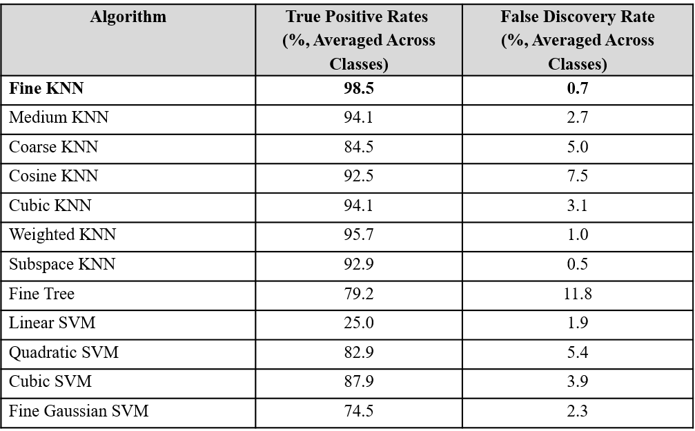
Once all data sets were synchronized, labelled, filtered, and normalized, the Fine k nearest neighbor (k-NN) classification algorithm provided by MATLAB was used to classify the data using a leave-one-out cross validation method. This was accomplished by training the algorithm on all datasets except for one, and then testing the algorithm on the “left-out” dataset. This test produced a set of algorithm-predicted labels for each row of the “left out” dataset. The Fine k-NN algorithm was utilized over other possible classification algorithms because when applied to the data in MATLAB’s classification learner add-on, the Fine k-NN algorithm achieved the highest reported classification accuracy (Table 1).

Table 1: Comparison of classification accuracy on all subject data using various classification algorithms. Multiple types of MATLAB classification algorithms were trained and tested using a leave-one-out cross validation method, and the mean classification accuracy rate for each classification algorithm were compared. The fine k nearest neighbor algorithm provided highest true positive rates and lowest false positive rate, and was therefore chosen for subsequent analyses.

To calculate the number of repetitions a subject performed of each exercise, data corresponding to Exercise 1, Exercise 2, and Exercise 3 were separately extracted from each dataset according to the column of algorithm-predicted discrete labels, and new tables of each activity were created for each subject. The MATLAB findpeaks function was then applied to different variable signals in each of these extracted activity tables to count the number of repetitions for each activity. For the Exercise 1 (elbow flexion/extension) tables, the x-axis accelerometer data from the forearm sensor was used, because clear peaks representing Exercise 1 repetitions are found in this data. For the same reason, the y-axis and x-axis gyroscope signal from the dorsal hand sensor were used to count repetitions of Exercise 2 and 3, respectively. An example of this process, as well as the previously mentioned data pre-processing methods, are shown in Figure 2.

Peak Counting Accuracy Calculation

To determine peak counting accuracy, the system’s estimate of the number of repetitions performed by the patient for each exercise, N_automatic, was compared to the repetition number as reported by the study personnel, N_manual. To calculate this accuracy, the percent error was calculated for each count and subtracted from 100%, according to the following formula:

Participants

Thirteen of the subjects enrolled in this study were healthy controls with no UE weakness (average age: 43 years old, range: 20 to 79 years old). Twenty subjects with recent stroke initially consented to the study, but four were excluded because they were unable to perform the three selected exercises (either due to somnolence or due to the affected arm being too weak to engage in multiple repetitions of the preselected exercises). Three subjects’ data were excluded because of incomplete data (due to sensor falling off during the session). In the end, 13 subjects with recent stroke completed the study. Of the 13 subjects whose data were used, mean age was 70 years old (range 40 to 90 years old), mean MRC scale score was 3.83, and mean time since stroke onset was 7.8 days.

Study Protocol Deviations, Technical Issues, and Adverse Events

Study sessions were monitored for complications such as accidental sensor removal during recording periods, skin irritation due to prolonged/repeated sensor placement, and allergic reactions to the adhesive material on the sensors. All subjects completed their testing time, no subjects reported skin irritation or allergic reactions to the sensors at any point during their participation in the study, and subjects typically found the sensors to be unnoticeable in terms of their comfort. However, there were six recording sessions in which accidental sensor removal did occur due to adhesive failure. When accidental sensor removal did occur, the resultant data set was either not used (three subjects) or re-recorded from the subject at a different time (three other subjects).

Comparison of Classification Accuracy between MATLAB Classification Algorithms

To determine which MATLAB classification algorithm would be best for the automatic repetition counting system, several MATLAB classification algorithms were applied to each of the data sets that included gyroscope and accelerometer data, and the average classification accuracies were compared [Table 1]. The Fine KNN or k-NN algorithm achieved the highest classification accuracy rates out of the relevant options.

Comparison of Repetition Counting Accuracy for Control and Stroke Patient Data Sets

Repetition Count Accuracy was compared between data obtained from healthy controls and data from stroke patients, who often may have higher variability in exercise performance due to weakness. With only accelerometer data used, the mean accuracy for healthy control data sets is 76.1 21.5 %, while the mean accuracy for the stroke patient data sets is 72.3 24.8 %. There was no significant difference between the two groups (p = 0.67). For the data sets with gyroscope data, the mean accuracy for healthy control data sets is 96.2 2.4 %, and the mean accuracy for the stroke patient data sets is 95.0 2.3 %, and no individual had accuracy lower than 94% [Table 2]. No significant difference was found between the control and stroke patient groups (p = 0.48).

Table 2: Exercise repetition counting accuracy in individual subjects. In subjects that had both accelerometry and gyroscopy data collected, the repetition count accuracy was similar in healthy controls and patients with mild/moderate (medical research council (MRC) strength score of 3/5 or 4/5 in the biceps and wrist extensors/flexors).

*Subject*	*Medical Research Council (MRC) Strength Scale Score*	*Accuracy (%)*
1	3	95.2
2	3	94.1
3	3	94.3
4	4	95.9
5	5/Healthy Control	96.2
6	5/Healthy Control	95.1
7	5/Healthy Control	95.8
8	5/Healthy Control	97.8

Comparison of Data Acquisition and Data Analysis Strategies

To determine if recording gyroscope data in addition to accelerometer data improved accuracy, the accuracy of data sets with gyroscope data was compared to those without. The mean accuracy for subject datasets with only accelerometer data is 74.6 22.8 %, while the mean accuracy for datasets that had both accelerometer and gyroscope data is 95.6 ± 2.4 %.

To ensure that this large discrepancy in accuracy is due to the effect of adding gyroscope data to the analysis and not due to variability between subjects, accuracy with and without gyroscope data were compared for each subject who had both accelerometer and gyroscope data collected. The overall mean accuracy without gyroscope data for these subjects is 84.3 18.0 %, compared to a mean accuracy of 95.6 ± 2.3 % for the same subjects when also using their gyroscope data. In every subject who had both accelerometry and gyroscopy data collected during the study session, adding gyroscope data to accelerometry data improved repetition counting accuracy (Fig. 3).

Effect of Number of Sensors

Using the parallel coordinates plot in MATLAB, we evaluated the relevance of the different variables in terms of classification accuracy (discrimination between the exercises) and found that the gyroscope + accelerometer data from the hand sensor and the accelerometer data from the forearm sensor are the most important variables for activity classification. Additionally, the findpeaks function performs most accurately when used on the x-axis accelerometer data from the forearm sensor or x-axis gyroscope data from the hand sensor for Exercise 1, the y-axis gyroscope data from the hand sensor for Exercise 2, and the x-axis gyroscope data from the hand sensor for Exercise 3. These findings suggest a relative sensor importance of Dorsal Hand > Forearm > Upper Arm (Brachium) sensor. Accordingly, when reducing the number of sensors, we decided to remove the upper arm sensor when limiting to two sensors and the upper arm and forearm sensor when limiting to one sensor. The additional testing to determine the accuracy of the systems with reduced sensor data was only performed for subjects from which gyroscope data was recorded. The mean accuracy for the system is 95.6 ± 2.4 % when incorporating data from three sensors, 92.7 6.6 % when using two sensors, and 85.1 11.9 % when using one sensor. (Fig. 4)

Effect of Forearm Sensor Placement

To ensure that the forearm sensor could be placed on either the flexor or extensor digitorum muscles and achieve similar levels of accuracy, the overall accuracies for all subjects with flexor and extensor sensor placements were compared. Since a larger number of the datasets that include gyroscope data used the flexor digitorum sensor position, only the accelerometry data from all datasets was used. The mean accuracy across all subjects with the forearm sensor in the flexor position is 76.8 19.1 %, and from the extensor position, 72.0 26.6 %. In order to determine if this difference in accuracy is statistically significant, a 2 sample T-test was performed (p = .58). This result indicates that there is not a statistically significant difference between the two sensor placements, and either forearm sensor position is viable for the system.

This study demonstrates the feasibility of using body-worn sensors to identify specific exercises and automatically count exercise repetitions in the inpatient stroke and acute rehabilitation setting. It also explores the effect of using different recording parameters on repetition count accuracy. While our study focused on three common upper extremity exercises, the conclusions on feasibility, data analysis approaches, and recording parameters provides insight for the design of future systems for exercise dose tracking.

In our 13 healthy controls and 13 inpatient hospital subjects with recent stroke, the sensors were well tolerated, and no subjects reported skin irritation or other side effects. However, there were several instances of skin adherence failures, when the adhesive sticker failed to keep the sensor on the subject’s arm for the entire duration of the study. Possible future solutions to this issue include using more adherent adhesives, although this will likely also increase patient discomfort with sensor removal. We have also found self-adherent (cohesive) bandages helpful when used in addition to the sensor adhesives.

Reducing the number of sensors per arm from three to two or one significantly reduced repetition counting accuracy, while adding gyroscope data collection significantly improved accuracy—especially in subjects with UE weakness due to stroke. In these patients, adding gyroscope recording to the dorsal hand sensor improved repetition count accuracy by over 10% (84.3 to 95.6%). Healthy subjects did not show such a large improvement in accuracy with the addition of gyroscope data, which may be due to a ceiling effect as healthy subjects had higher repetition accuracy with accelerometry alone. This may be because gyroscope data measures rotation about an axis, and like many exercises from the stroke rehabilitation regimen, the three exercises we chose for our study are rotational “range of motion” exercises. This suggests that gyroscopy is likely an important measurement to capture in future studies monitoring stroke rehabilitation efforts.

On all subjects from whom gyroscope data was recorded, an overall repetition-counting accuracy of at least 94.1% was achieved, even for patients with an MRC strength scale score of 3/5. The system’s repetition counting was more accurate when gyroscope data was recorded and implemented in addition to accelerometer data. The system’s repetition counting became less accurate as fewer sensors’ inputs were utilized, and the best performance was achieved using all three sensors’ data.

While the results of this study are promising, there are several limitations. First, the system has only been tested on three basic exercises in terms of classification and repetition counting ability. Secondly, all incorporated stroke patient data was collected from subjects with an MRC strength scale of 3 or greater (moderate UE weakness or better), which does not represent the entire population of patients with stroke. Therefore, the system’s ability to successfully quantify exercise dosage of a wider range of UE exercises and/or from patients with greater UE weakness is uncertain. More advanced data science techniques may help overcome some of the challenges related to variability of movements in patients with weakness due to stroke. For example, the method for counting exercise repetitions used a readily available Fine k nearest neighbor algorithm. Alternative time-series analysis approaches that can take into account the temporal progression of movements involved in an exercise may help identify movement patterns with a wider range of speeds or movement pauses.

Finally, the current system has recording time restraints due to battery limitations. For example, adding gyroscope data in addition to accelerometer data reduces the recording time of the current sensors from 21 hours to only three hours (if both data are recorded with a 62.5 Hz sampling rate). Longer-term monitoring studies will require longer-lasting sensor batteries or more conservative recording solutions.

In recent years, multiple studies have been published reporting the use of similar sensor systems for automated movement tracking, with the majority of these studies focusing on the classification of whole-body movements, such as standing, sitting, walking, ascending/ descending stairs, playing sports, cycling, and others.^16,17 Classification of UE movements have been more limited in scope and/or application of the system. Biswas et al. and Bochniewicz et al. built classification algorithms for UE exercises and applied them to stroke patient data, but did not attempt to create a repetition quantifying system to measure exercise dose.^14,15 Other examples, such as Zhang et al. and Crema et al., created UE exercise classification and repetition counting systems but did not apply them to data from patients.^18,19 More recently, Guerra and colleagues developed a movement classification system that could be used to enumerate repetitions and applied the system to stroke patient data with a focus on the classification of movement primitives (components of UE movements that cannot be broken down further). They report lower rates of accuracy (precision of approximately 80% in control patients, 79% in patients with weakness due to stroke) than in our study.²⁰ While specifics about the particular UE movements studied (exercises versus movement primitives) may have contributed to this observed difference in accuracy, it is important to note that we also used a different categorization and repetition counting strategy. In our algorithm, activity is first classified and then number of repetitions is estimated by counting peaks in data from the sensor that was previously seen to have maximum fluctuations during the course of the exercise. Such a strategy is less sensitive to classification errors, and thus has higher repetition counting accuracy. Future work will investigate the success of both strategies when applied to more types of exercises and a wider range of patient data.

In summary, this work suggests that using wearable sensors in the inpatient stroke and acute rehabilitation setting is feasible and has the potential for creating an automated system to quantify individual rehabilitation therapy dose. Future work is needed to expand the range of rehabilitation activities identified by this system and to improve sensor adherence and battery life. Ultimately such a system may contribute to answering key questions about how patient exercise “dose” in the acute/subacute period post-stroke affects final motor outcomes, produce a system for providing patient feedback on how their efforts compare to target doses, and improve patient post-stroke function.

Ethics Approval and Consent to Participate

The study protocol was approved by the Research Subjects Review Board of the University of Rochester (RSRB STUDY00001668), and all subjects signed a written informed consent document prior to starting study procedures.

Consent For Publication

Not applicable.

Authors’ Contributions

NB provided input on the study’s design, approached subjects to ask for their consent to participate, recorded data from subjects, performed data processing and analysis, and contributed to the writing of the manuscript and creation of the figures. GS provided expertise on the usage of the sensors and data processing strategies, and critical review of the manuscript. LR provided expertise on the study’s design, input on exercise selection, and critical review of the manuscript. AB conceptualized and modified the study’s design, approached subjects to ask for their consent to participate, recorded data from subjects, and contributed to the writing of the manuscript and creation of the figures.

Funding Disclosures

AB was supported by the following grants: NRSA 2T32NS007338-16 (NIH) and the NTRAIN K12 program (NIH/NICHD 1K12 HD093427-01). This project is also supported by a pilot grant from the University of Rochester CHeT Institute. None of the aforementioned entities were involved in the design, analysis, interpretation of data, or writing of the manuscript for the study.

Competing Interests

MC10 Inc. provided the sensor equipment (BiostampRC sensors) as a research grant to AB. MC10 Inc. was not involved in the design, analysis, interpretation of data, or writing of the manuscript for the study.

Availability of Data and Materials

The datasets used and analysed during the current study are available from the corresponding author on reasonable request.

Acknowledgements

We would like to thank Simon Carsen, Tanzeem Choudhury and Kyle Choi for their contribution of advice and support, and the URMC neurology department residents, nursing staff, and occupational and physical therapists for their input, assistance with recruiting subjects, and their accommodation of the collection of data for the study. We would also like to thank Solomon Abiola for initial discussions on potential uses of sensor technologies, and Paige Hepple and Robert Holloway for helpful comments on the manuscript.

Benjamin EJ, Muntner P, Alonso A, et al. Heart Disease and Stroke Statistics-2019 Update: A Report From the American Heart Association. Circulation. 2019. doi:10.1161/CIR.0000000000000659
Gadidi V, Katz-Leurer M, Carmeli E, Bornstein NM. Long-term outcome poststroke: Predictors of activity limitation and participation restriction. Arch Phys Med Rehabil. 2011;92(11):1802-1808. doi:10.1016/j.apmr.2011.06.014
Winstein CJ, Stein J, Arena R, et al. AHA / ASA Guideline Guidelines for Adult Stroke Rehabilitation and Recovery.; 2016. doi:10.1161/STR.0000000000000098
Winstein CJ, Stein J, Arena R, et al. Guidelines for Adult Stroke Rehabilitation and Recovery. Stroke. 2016. doi:10.1161/STR.0000000000000098
Kwakkel G, Lannin NA, Borschmann K, et al. Standardized measurement of sensorimotor recovery in stroke trials : Consensus-based core recommendations from the Stroke Recovery and Rehabilitation Roundtable. 2017;12(5):451-461. doi:10.1177/1747493017711813
Langhorne P, Wagenaar R, Partridge C. Physiotherapy after stroke: more is better? Physiother Res Int. 1996. doi:10.1002/pri.6120010204
Kwakkel G, Van Peppen R, Wagenaar RC, et al. Effects of augmented exercise therapy time after stroke: A meta-analysis. In: Stroke. Vol 35. ; 2004:2529-2536. doi:10.1161/01.STR.0000143153.76460.7d
Galvin R, Murphy B, Cusack T, Stokes E. The impact of increased duration of exercise therapy on functional recovery following stroke--what is the evidence? Top Stroke Rehabil. 2008;15(4):365-377. doi:10.1310/tsr1504-365
Lohse KR, Lang CE, Boyd LA. Is more better? Using metadata to explore dose-response relationships in stroke rehabilitation. Stroke. 2014;45(7):2053-2058. doi:10.1161/STROKEAHA.114.004695
Bernhardt J, Hayward KS, Dancause N, et al. A Stroke Recovery Trial Development Framework: Consensus-Based Core Recommendations from the Second Stroke Recovery and Rehabilitation Roundtable. Neurorehabil Neural Repair. 2019;33(11):959-969. doi:10.1177/1545968319888642
Lang CE, Macdonald JR, Reisman DS, et al. Observation of amounts of movement practice provided during stroke rehabilitation. Arch Phys Med Rehabil. 2009;90(10):1692-1698. doi:10.1016/j.apmr.2009.04.005.Observation
Valevicius AM, Jun PY, Hebert JS, Vette AH. Use of optical motion capture for the analysis of normative upper body kinematics during functional upper limb tasks: A systematic review. J Electromyogr Kinesiol. 2018. doi:10.1016/j.jelekin.2018.02.011
Arac A, Zhao P, Dobkin BH, Carmichael ST, Golshani P. Deepbehavior: A deep learning toolbox for automated analysis of animal and human behavior imaging data. Front Syst Neurosci. 2019. doi:10.3389/fnsys.2019.00020
Biswas D, Corda D, Baldus G, et al. Recognition of elementary arm movements using orientation of a tri-axial accelerometer located near the wrist. Physiol Meas. 2014;35(9):1751-1768. doi:10.1088/0967-3334/35/9/1751
Bochniewicz EM, Emmer G, McLeod A, Barth J, Dromerick AW, Lum P. Measuring Functional Arm Movement after Stroke Using a Single Wrist-Worn Sensor and Machine Learning. J Stroke Cerebrovasc Dis. 2017;26(12):2880-2887. doi:10.1016/j.jstrokecerebrovasdis.2017.07.004
Altun K, Barshan B, Tunçel O. Comparative study on classifying human activities with miniature inertial and magnetic sensors. Pattern Recognit. 2010. doi:10.1016/j.patcog.2010.04.019
Attal F, Mohammed S, Dedabrishvili M, Chamroukhi F, Oukhellou L, Amirat Y. Physical human activity recognition using wearable sensors. Sensors (Switzerland). 2015. doi:10.3390/s151229858
Zhang Z, Fang Q, Ferry F. Upper limb motion capturing and classification for unsupervised stroke rehabilitation. In: IECON Proceedings (Industrial Electronics Conference). ; 2011. doi:10.1109/IECON.2011.6119934
Crema C, Depari A, Flammini A, Sisinni E, Haslwanter T, Salzmann S. Characterization of a wearable system for automatic supervision of fitness exercises. Meas J Int Meas Confed. 2019. doi:10.1016/j.measurement.2019.07.038
Guerra J, Uddin J, Nilsen D, et al. Capture, learning, and classification of upper extremity movement primitives in healthy controls and stroke patients. IEEE Int Conf Rehabil Robot. 2017:547-554. doi:10.1109/ICORR.2017.8009305

Download PDF

Journal Publication

published 02 Jul, 2021

Read the published version in Digital Biomarkers →

Version 1

posted

You are reading this latest preprint version

Automatic Identification of Upper Extremity Rehabilitation Exercise Type and Dose Using Body-Worn Sensors and Machine Learning: A Pilot Study

Status:

Journal Publication

Version 1

Abstract

Figures

Introduction

Methods

Results

Discussion

Conclusions

Declarations

References

Status:

Journal Publication

Version 1