Patient specific 3D finite element model was constructed from CT images data of AIS. The correction effects of different applied forces were analyzed by using biomechanical principles.
Personalization of the finite element model
The patient was an 11 year old with AIS, having typical right thoracic and left lumbar scoliotic curvatures, with thoracic Cobb angle of 36° and lumbar Cobb angle of 24°. The maximum lateral bending displacement was in T9 and L3 vertebrae. In coronal plane, displacements were 63mm and 32mm whereas in sagittal plane these were 46mm and 35mm respectively. The maximum rotation angle of ribs was 13° and kyphotic displacement of ribs was 23 mm. A 3D model of AIS was established by using medical image processing software (Mimics 19.0; Materialise, Leuven) from DICOM CT images. Spine model was extracted according to bone threshold and then region growing tool was used to segment the different regions. According to the knowledge of human anatomy, a three-dimensional model of AIS including the thoracolumbar vertebrae, intervertebral disc, ribs and pelvis was established. By comparing the finite element model with the patient's X-ray film, the distance between the length of the vertebral mass and the tibia and the distance between the X-ray films are less than 1 mm. The angle between the midline of each vertebra and the tibia and the angle between the X-ray films are less than 0.5 degrees. This proves that the model is basically consistent with the patient's scoliosis features. Point cloud data was obtained by scanning patient's body surface with a 3D scanner. In Geomagic studio we denoised and smoothened to reconstruct a 3D model of body contour. Patient's body surface was assembled with its skeletal model to obtain 3D geometric model of trunk. The software (Hypermesh13.0; Altair; America) was used to mesh 3D model.
A personalized model contains 152301 nodes and 302357 tetrahedral elements representing the thoracic and lumbar vertebrae, intervertebral disks, ribs, sternum, intercostal ligaments, anterior longitudinal ligament, posterior longitudinal ligament, ligamentum flavum, intertransverse ligaments, interspinal ligament, supraspinal ligament, costovertebral and costotransverse joints, and zygapophyseal articulations. Muscle tissues (trapezius muscle, abdominal muscles, rectus muscle and so on) were simulated by spring elements. Mechanical properties of anatomical structures were taken from published data (see Table 1) [10, 13-16]. Finally 3D model was processed and simulated in CAE (computer assisted engineering) software (Abaqus 6.14-2; Dassault; France) to simulate.
Objective function
Due to symmetry of human body, there is no hump in coronal plane of the normal spine and ribs are symmetrically in horizontal plane of midline of spine [17]. In order to obtain curve of normal spine in sagittal plane, 12 healthy adolescents with no medical history of spinal disorders were selected, with an average age of 12.0 years consisting of 6 males and 6 females. The results in form of normal curve of spine were obtained.
Defining parameters
In coordinate system, coronal axis was X axis, sagittal axis Y axis and vertical axis as Z axis. Curvature curve was defined by connecting the center of each vertebral body in 3D model. Similarly, normal spinal curve was defined. In this work, objective function was consisted of seven variables; displacement distance between scolitic and normal spinal curves in thoracic and lumbar regions in coronal plane as X1, X2, and in sagittal plane as Y1, Y2 respectively. Distance between left and right ribs kyphosis in horizontal plane was defined as C. The rotation angle of first scoliosis rib was θz0, and initial rotation angle of vertebral body was θy0. These variables are represented in the 3D view interface as shown in Fig. 1.
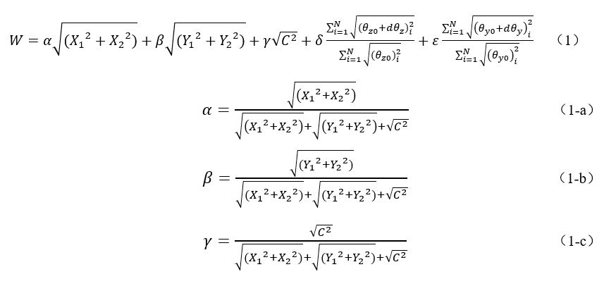
Since geometric variables may be positive or negative, the square of displacement was chosen to be square and square root to ensure that the numerical value is positive. The objective function is expressed as follows:
See Formula 1 in the Supplementary Files.
Where α, β, γ and δ, ε are the weightings of distance and rotation in coronal, sagittal and horizontal planes respectively.
The interval ranges from 0 to 1, N is total number of vertebrae, and dθ is increment of relative initial rotation value of each vertebra. In order to fully consider the lateral bending of vertebrae and ribs, rotation angles of each rib and vertebrae were counted. The optimal solution of objective function was to reach the minimum value that is 0 in equation.
The optimal scoliosis correction curve was considered when body was in upright position whereas lateral displacement, tilt angle and axial rotation of spine in 3D space were all 0. In actual clinical scoliosis correction process, due to complexity of muscles, skeleton and other structures, the correction often cannot achieve ideal state. Therefore, in treatment of scoliosis, goal is to minimize the objective function. It can be done to minimize each variable in space as much as possible. In patients with bilateral bends, displacement of coronal plane is statistically larger than that of sagittal plane [11]. Clinically, physicians usually consider coronal deviation. Instead of vertebral rotation, ribs rotation angle is smaller. In order to distribute the weight of each variable reasonably, which is to define the proportion of each deformation amount to the total deformation amount. Larger the migration distance, larger the weight.
Loading condition
Three point force principle is applied to scoliosis model to achieve correction effects in 3D space. Applied force was divided into three groups: a. F1 and F2 were applied to thoracic vertebrae and ribs to examine correction of thoracic vertebrae in coronal axis and ribs kyphosis. b. Application of F3 and F4 in position of lumbar scoliosis, measuring lumbar vertebral correction; c. Four sets of correction forces, F1, F2, F3 and F4, were applied to position of lateral bend at same time. In coronal plane, F1 and F3 correction forces were applied to thoracic and lumbar vertebrae in coronal plane. In horizontal plane, deformity of vertebral rotation was improved by applying F2 correction forces on kyphotic ribs. In sagittal plane, F4 correction forces were applied to posterior lumbar spine to alleviate flat back and to maintain normal physiological curvature. The specific application of force is shown in Fig. 2. Proposed forces were transmitted to spine through thoracic and lumbar soft tissues.
Review of literature concerning non-surgical treatment of scoliosis showed that initial maximum displacement of thoracic and lumbar vertebrae is within 100 mm and rotation angle of ribs is within 40° [18]. In order to make this study more practical, the maximum displacement of vertebrae and maximum rotation angle of ribs were set at 200 mm and 50° respectively.
Finite element analysis
When body is under high pressure, it will not only produce discomfort but also cause pressure ulcers. In order to ensure that local pressure is within tolerance range, it is necessary to select a reasonable stress area. Visser D et al [19] used visual analogue scales and pressure sensors to measure pressure generated by braces. Other researchers measured pressure on trunk of in-braces patients in range of 10 cm2 and withstanding 10 Kpa pressure while contact point force was kept within 10 N, [20-22]. Cobetto et al [23] collected the pressure between brace and patient's body surface and gave a withstanding threshold of 35 Kpa. The correction forces were guaranteed in range of human pain threshold. The applied range of force was 0 ~ 100N, and the applied area was 64 ~ 225 cm2 [23,24].
Convergence conditions
Internal and external geometries were linked together. Using an iterative nonlinear resolution method, applied forces on selected vertebrae lead to correction of external trunk model [24,25]. The simulation boundary conditions included a fixed pelvis in rotation-translation. T1 was limited to transverse plan movements. According to scoliosis curve of patient, the values of variables in objective function were calculated, and initial variables were taken as original values. By adjusting magnitude of correction forces, the deformation of objective function was obtained. As the initial value of next iteration, results of the previous step were iterated until convergence conditions were satisfied. Convergence conditions used were as: 1. total number of iterations exceeding 200 steps; 2. variation of variables in two iterations was within 2mm; 3. difference between two iterations was less than 1 N, accounting for about 1% of the force range. When convergence condition was reached, the iteration was terminated.