Geomagnetism, similar to other areas of geophysics, is an observation-based science. Data agreement between comparative geomagnetic vector observations is one of the most important evaluation criteria for high-quality geomagnetic data. The main influencing factors affecting the agreement between comparative observational data are the attitude angle, scale factor, long-term time drift, and temperature. In this paper, we propose a method based on a genetic algorithm and linear regression to correct for these effects and use the distribution pattern of points in Bland–Altman plots with a 95% confidence interval length to qualitatively and quantitatively evaluate the agreement between the comparative observational data. In Bland–Altman plots with better agreement, that is, with the corrected data, more than 95% of the points are distributed within the 95% confidence interval and there is no obvious pattern in the distribution of the points. Meanwhile, the length of 95% confidence interval decreased significantly after the correction. The method presented here has positive effects on the vector instrumentation detection, enhancing the robustness of comparative observatory observations and reducing errors in judgments of the size and arrival time of large magnetic disturbances or rapid magnetic variations.
Research Article
Data Agreement Analysis And Correction of Comparative Geomagnetic Vector Observations
https://doi.org/10.21203/rs.3.rs-970823/v1
This work is licensed under a CC BY 4.0 License
Journal Publication
published 11 Feb, 2022
You are reading this latest preprint version
Vector observations of the geomagnetic variation field are the primary means used to study internal and external magnetic field sources, such as rapid magnetic variations and magnetospheric currents (Curto 2007; Xu 2015), and the instrument most commonly used for such observations is the fluxgate magnetometer (Jankowski and Sucksdorff 1996). To enhance the operational robustness, some observatories use two sets of fluxgate magnetometers with the same type of probe to enable comparative observations. However, actual comparative observational data can be somewhat divergent, that is, the measurement data from the two sets of instruments do not exactly agree. This leads to a reduction in the credibility of the data recorded by one instrument when the other fails, to the point where it is impossible to determine whether it is reasonable to use the data from the backup instrument at the time of failure. Furthermore, because vector observations of the geomagnetic field are expected to qualitatively reflect the magnetic field variations at the measurement points and therefore to invert the relevant physical mechanisms, morphological differences in the comparative observational data increase, to some extent, the difficulties associated with determining the arrival time and the magnitude of large magnetic disturbances (Araki et al. 2004; Segarra and Curto 2013). Therefore, analyzing and correcting the agreement between the comparative geomagnetic vector observational data are basic but important tasks.
Morphological differences in the comparative geomagnetic vector observational data have a variety of causes. For fluxgate magnetometers with the same type of probe, influencing factors that can introduce significant magnetic measurement differences include the attitude angle, scale factor, long-term time drift, and temperature. For daily variations, the attitude angle and the scale factor cause the geomagnetic vector difference to show a characteristic pattern. The effects of the long-term time drift and temperature are more often seen in long-term observations. In China, most geomagnetic observatories have a strict temperature control of 0.04 °C/day in their variation rooms. The variation rooms of the three Chinese geomagnetic observatories selected for this study all meet this requirement. Therefore, when examining the agreement between the daily-variation data, only two aspects—the attitude angle and the scale factor—are analyzed. For long-term observations (greater than or equal to 3 months), the effects of the long-term time drift and temperature cannot be neglected.
The traditional index for evaluating the agreement between comparative geomagnetic vector observational data is the Pearson correlation coefficient (Han et al. 2004; Berezin and Tlatov 2020). This correlation coefficient gives a clear agreement judgement when comparing measurement data from two different means of observation (e.g., satellite magnetic observations versus ground-based observations). When the measurement platform is consistent, the observational environment is good, the instrument quality is high, and the correlation coefficient is often very close to 1. However, the geomagnetic vector differences can still be relatively large and show some regularity. This means that the correlation coefficient does not adequately distinguish the degree of agreement between the comparative observational data. This paper proposes a qualitative and quantitative analysis of the agreement between comparative geomagnetic vector observational data using Bland–Altman (B–A) plots. Disagreement can be visually detected from the shape of the distribution of the points on the B–A plots, and the length of the 95% confidence interval can significantly distinguish the superiority or inferiority of the agreement.
To analyze the influencing factors affecting the agreement between the comparative geomagnetic vector observations and to calculate the corresponding correction parameters, the Lijiang (LIJ), Maguan (MAG), and Yunlong (YUL) geomagnetic observatories in southeastern China, which have two sets of fluxgate magnetometers operating simultaneously, were selected. These three observatories are equipped with two sets of GM4 fluxgate magnetometers with a resolution of 0.01 nT and a sampling rate of 1 Hz. The selected data range is from January 1, 2020, to July 31, 2021.
Attitude angles are important for geomagnetic vector observations. Traditionally, the determination of the azimuth of the fluxgate magnetometer by the staff is made in conjunction with the fluxgate theodolite according to the geographical orientation (Jankowski and Sucksdorff 1996). The tilt of the instrument above the abutment is recorded in real time using a high-precision tiltmeter or a suspended fluxgate magnetometer to circumvent the effect of the tilt. However, in practice, tilt effects are often ignored for observatories in non-permafrost environments. Unattended platforms, such as the SeaFloor ElectroMagnetic Station, use direct attitude measurements by means of tiltmeters and fiber optic gyroscopes (Toh et al. 2006). Researchers have also tried to correct the attitude between two fluxgate magnetometers using genetic algorithms (Liu et al. 2019). A genetic algorithm is a computational model that simulates the process of natural selection and genetic evolution observed in biological evolution; this is a well-established method for finding the global optimal solution of an objective function (Holland 1992; Weile and Michielssen 1997). Earlier studies have used genetic algorithms to calibrate the orthogonality of fluxgate magnetometer probes (Jiao et al. 2011). Three-component fluxgate magnetometer data naturally contain attitude information, and ideally the difference in the data between the two sets of instruments only arises from the difference in the attitude angles. Accordingly, the genetic algorithm calculates the attitude relationship between two fluxgate magnetometers and has natural advantages such as high measurement accuracy, no interference with the probe, and a minimal use of peripheral instruments.
The objective function of the genetic algorithm used in this paper is the difference between the value of the tested instrument data normalized to the standard instrument coordinate system and the value of the standard instrument data, as shown in Equation (1).

In Equation (1), the subscripts standard and test represent the data in the standard coordinate system and in the tested coordinate system, respectively, and the superscript ' represents data converted from another coordinate system. The rotation matrix T is obtained by multiplying the rotation matrices represented by the tilt angles Roll, Pitch, and the heading angle Yaw in sequence during the conversion from the standard coordinate system to the tested coordinate system, as shown in Equation (2).

This order cannot be changed because the attitude angles correspond to the rotation angles only when the matrix is multiplied in this order.
The presence of deviations in the attitude angles between the two fluxgate magnetometers results in a geomagnetic vector difference in one direction, reflecting a morphological change in the other direction due to projection (Wang et al. 2017). Taking the deviation of the heading angle Yaw as an example, as in Figure 1, the difference dH of the H component reflects the morphological variation of the D component.
Even for the same probe, the characterization factor, that is, the scale factor, used to convert the voltage to the magnetic induction intensity during the instrument commissioning process is not the same. Therefore, the scale factor matrix also needs to be added to the objective function, as in Equation (3).

Here, the matrix Sf is the scale factor matrix, which is a diagonal array with its diagonal elements being the scale factors of the corresponding components. The scale factor naturally exists and acts on the tested instrument data first, as in Equation (4); therefore, the attitude rotation matrix and the scale factor matrix acting on the tested instrument data are not interchangeable.

Note that the attitude angle and scale factor parameters are for the instrument being tested relative to the standard instrument. The positive direction of the angle is a counterclockwise rotation around the rotation axis, and each scale factor consists of the tested instrument data divided by the standard instrument data.
The presence of the scale factor between the two instruments results in a geomagnetic vector difference in one direction, reflecting a morphological change in this same direction. As shown in Figure 1, the D component difference, dD, exhibits its own morphological variation, that is, it exhibits the morphological variation of the D component.
In the literature (Liu et al. 2019), after selecting the appropriate genetic algorithm parameters, the tested instrument data are first obtained by an angular rotation of the standard instrument data and then a genetic algorithm is used to calculate the attitude angle between the data with an accuracy of up to 10−4 nT(the maximum absolute value of the difference).We can make slight improvements by running each attitude angle calculation 10 times; then, after excluding results that are more than one standard deviation from the mean, the mean value can be used as the attitude angle solution to further constrain the convergence of the genetic algorithm solution. In this way, the maximum absolute difference between the tested instrument data and the standard instrument data after the attitude angle correction can reach 10−5 nT.
Actual observations are often not so ideal. During the period of June 2–July 15, 2021, we conducted related experiments at the LIJ. Two sets of fluxgate magnetometers of the same type were used to make comparative observations. The standard instrument and the tested instrument were spaced 7-m apart, and both were placed on a stone pier in the variation room, with a deviation of 30° in the heading angle between the two. The 7 days with the smallest standard deviation for the results calculated by the genetic algorithm were taken, and the results are shown in Table 1.
Table 1. Calculated results of the comparative attitude angle observation experiment.
|
No. |
Roll (°) |
Pitch (°) |
Yaw (°) |
|
1 |
-2.211 |
-0.437 |
30.000 |
|
2 |
-0.831 |
-4.140 |
30.000 |
|
3 |
-1.978 |
2.434 |
30.000 |
|
4 |
-0.984 |
0.791 |
29.997 |
|
5 |
-0.512 |
1.158 |
29.943 |
|
6 |
-1.192 |
1.060 |
29.942 |
|
7 |
-1.050 |
1.545 |
29.907 |
|
Average |
-1.251 |
0.345 |
29.970 |
|
Standard deviation |
0.572 |
1.997 |
0.035 |
The calculated heading angle of 29.970° is very close to 30° with a small standard deviation of 0.035°, which indicates that the method used here is able to calculate large existing angles between two fluxgate magnetometers with high accuracy. However, smaller angles, where the standard deviation of the calculated angles over multiple days is greater than the mean value, need to be considered separately.
In the comparative geomagnetic vector observations, the static attitudes of the two fluxgate magnetometers often differ to some extent. Furthermore, the vector difference between the tested instrument data and the standard instrument data after the attitude angle correction is stabilized within approximately 0.5 nT. This requires that the standard deviation of the calculated angle be less than 0.057° (e.g., for a residual magnetic field of 100 nT). However, this requirement is not always satisfied as a result of the quality of the data or disturbances in the observational environment. Therefore, when designing the correction process, we chose, as the criterion to judge the correct calculation of the attitude angles, the uncertainty of all three angles of the multi-day calculation results to be less than 0.1° or the uncertainty of the calculation results of significantly large attitude angles (greater than 1°) to be less than 0.057°.
As for the scale factor, the calculated uncertainty (expressed as the standard deviation of the multi-day scale factors) is small. It is approximately 0.002 for observatories with a good observational environment, resulting in an uncertainty of less than 0.1 nT for the magnetic field. In this paper, after determining the relative attitude angles of the two instruments, we calculate the scale factor for each day in 3 consecutive months and perform linear regression to obtain the base scale factor (intercept) and the long-term time drift (slope). Instrumental scientists and engineers assume that the long-term time drift of a fluxgate magnetometer is linear (Gordon and Brown 1972; Esper 2020); such behavior is characterized by tiny fluctuations in the short-term observations and non-negligible and linear variations in the long-term observations. If the long-term time drifts of the two instruments are different, there will be a linear change in the scale factor between the instruments over time. This is a relative relationship and does not specify whether the drift comes from the tested instrument or the standard instrument or both. However, for the correction of the long-term observational agreement, it is sufficient to assume that the drift comes from the tested instrument.
Temperature has an important effect on fluxgate magnetometers (Primdahl 1979). New fluxgate magnetometers have been able to achieve a thermal drift of less than 0.1 nT/°C in the laboratory (Korepanov 2012). However, the effect of temperature on fluxgate magnetometers is still very important and non-negligible in long-term observations. Even though the temperature difference between two sets of instruments in the same variation room is nearly constant (the mean value of the temperature difference between the two sets of instruments at LIJ from January 1, 2020, to March 31, 2020, was 0.9672 °C, and the standard deviation was 0.0863 °C), the measurement difference caused by the fixed temperature difference is not constant, which means that the temperature change affects the measurement difference between the two sets of instruments. The top section of Figure 2 shows the Z component difference, dZ, and temperature variation of the two sets of instrumental data from January to March 2020 at LIJ after the attitude angle, scale factor, and long-term time drift corrections. The dZ pattern, showing a decrease followed by an increase, is very similar to the temperature variation. This relationship is approximately linear, as seen in the scatter plot of dZ versus temperature (middle section of Figure 2). The temperature, rather than the temperature difference, has a linear effect on the vector difference between the two sets of instruments. This can be interpreted as the difference in the temperature coefficients between the two sets of instruments leading to differences in the measurements at different temperature points (the red line at the bottom of Figure 2), even though the temperature difference is always constant (the blue line at the bottom of Figure 2).
The morphological differences and the data disagreement in the comparative geomagnetic vector observations are primarily due to the attitude angle, scale factor, long-term drift, and relative temperature coefficients. The calculations of the attitude angle and the scale factor are based on the genetic algorithm. The long-term time drift and relative temperature coefficients are then obtained via linear regression. The parameter calculation and correction flow used in this paper are shown in Figure 3.
The calculation results for the attitude angle and the scale factor based on the genetic algorithm are shown in Table 2.
|
YUL 2020/05-2020/07 |
Attitude angle (°) |
||
|
Roll(ave/std) |
Pitch(ave/std) |
Yaw(ave/std) |
|
|
0.487/0.087 |
0.421/0.097 |
-2.341/0.074 |
|
|
Scale factor |
|||
|
H |
D |
Z |
|
|
1.008585 |
0.980915 |
0.994477 |
|
|
LIJ 2020/01-2020/03 |
Attitude angle (°) |
||
|
Roll(ave/std) |
Pitch(ave/std) |
Yaw(ave/std) |
|
|
0.053/0.105 |
-0.018/0.148 |
-0.067/0.117 |
|
|
Scale factor |
|||
|
H |
D |
Z |
|
|
0.965424 |
1.002734 |
0.958902 |
|
|
MAG 2021/01-2021/03 |
Attitude angle (°) |
||
|
Roll(ave/std) |
Pitch(ave/std) |
Yaw(ave/std) |
|
|
-0.093/0.298 |
-0.147/0.681 |
-1.100/0.051 |
|
|
Scale factor |
|||
|
H |
D |
Z |
|
|
0.992251 |
1.002943 |
1.001010 |
|
Of the nine attitude angles shown in Table 2, only the three attitude angles of YUL and the heading angle of MAG are available because their mean values are large and their standard deviations are small. In particular, the computed mean values of the heading angles of the YUL and MAG exceed 1°, while their standard deviations are less than 0.057°. The remaining five attitude angles have average values close to 0 and standard deviations greater than the average. In the actual correction procedures, it was assumed that there was no angular deviation on the axis between the two sets of instruments. The calculation of the scale factor was performed after the attitude correction. The results of 3 consecutive months of calculations were linearly regressed after removing significantly erroneous data to obtain the intercept and slope, which were used as the scale factor and long-term time drift correction parameters, respectively.
The parameters used to correct the single-day data are the attitude angle and the scale factor. For the sake of brevity, the attitude angle and scale factor correction is called the daily correction. The attitude, scale factor, long-term time drift, and relative temperature coefficient correction is called the long-term correction. The daily correction differs from the long-term correction not only in the correction parameters but also in the demeaning operation of the data preprocessing. Because the geomagnetic vector observations are concerned with the variation of the geomagnetic field and the geomagnetic vector baseline is determined by other methods at the observatory, the mean value of each component needs to be subtracted from the raw vector data for the single-day correction; meanwhile, the long-term correction subtracts the mean value of the magnetic field corresponding to the length of the time series.
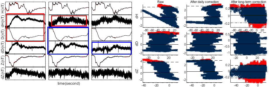
The daily-variation comparison curve of YUL on June 17, 2020, is taken as an example of the parameter calculation and the correction effect of the daily correction. The raw data are shown in Figure 4a. The morphology of dH is clearly similar to that of the D component, while the correlation with the H component itself is not obvious. This is a typical feature of morphological disagreements due to a heading angle deviation, which agrees well with the calculated result: a larger heading angle deviation between the two instruments (the Yaw angle at YUL is −2.341°). After just the attitude angle correction, as shown in Figure 4b, the morphological correlation between dH and D is weakened; however, the morphological correlation between dD and D is still strong. As shown in Figure 4c, the correlation between dD and D is weakened after performing the attitude angle and scale factor corrections. The maximum value of the geomagnetic vector difference is reduced from approximately 1.3 nT with the original data to approximately 0.5 nT after the daily correction.
Taking LIJ with its complete temperature measurements and small environmental disturbance as an example, a linear regression analysis of the long-term time drift and relative temperature coefficient over 3 months is shown in Figure 5. Note that the long-term time drift of the instrument is given in units of nT/day and is obtained by multiplying the slope of the scale factor by the amplitude of the daily variation (in the case of 30 nT). The residual magnetic field strength is not multiplied by the slope of the scale factor here because, when the instrument is misoriented or other factors cause the residual magnetic field strength of a component to be large, this will cause the calculated value of the long-term time drift to be too large. The effect of the long-term time drift varies from instrument to instrument and is generally not significant. However, the effect of temperature is more than was expected. Even though the D component appears to have two fitted straight lines, which are discussed below, the 3-month continuous temperature variation has a good linear relationship with the vector difference and a large slope of approximately 3 nT/°C, which is important for studies of the data agreement between long-term comparative observations.
The difference between the comparative observational data after the long-term correction is shown in Figure 6. It can be seen that, after the daily correction (Figure 6b), the daily variation of the geomagnetic vector difference is significantly reduced and its trend is consistent with that of the temperature. After the long-term correction (Figure 6c blue line), the dH and dZ variations are no longer temperature-dependent and do not have significant temporal patterns, showing flatter straight trends. Note that, in Figure 6b, dD deviates significantly from the temperature change after approximately 41 days (the thick red line) but its trend is still the same as that of the temperature, which leads to an increase in dD in the second half of Figure 6c, instead continuing as a straight line. This is believed to reflect the case in which a temperature inflection point causes a change in the trend, resulting in a change in the relative temperature coefficient of the probe pair on a certain component, as explained in detail in the discussion. From a quantitative point of view, the maximum value of the geomagnetic vector difference is reduced from approximately 3 nT to approximately 0.5 nT after the long-term correction.
B–A plots: a more appropriate method for data agreement evaluations of comparative geomagnetic vector observations
Traditionally, the data agreement between comparative geomagnetic vector observations is often expressed by the Pearson correlation coefficient. In the case where the comparison is between two different observation platforms or two sets of instruments on the same platform that are not precisely calibrated, the correlation coefficient can appropriately distinguish the degree of agreement in the trend of the comparative observational data. However, the resolution of ground-based observations made by currently available fluxgate magnetometers has increased significantly. With the precise orientation adjustments made by observatory staff and the strict temperature control available in geomagnetic variation rooms, the correlation coefficients of the comparative observations are often so high that they cannot adequately describe data disagreements.
Take LIJ as an example. Its correlation coefficient prior to the daily correction is generally higher than 0.9995, and the difference between the correlation coefficients before and after the correction is on the order of 10−15. Prior to the long-term correction, the correlation coefficients of all three components of the comparative observational data for 3 consecutive months were higher than 0.995 and the difference between the correlation coefficients before and after the correction is in the order of 10−11. This indicates that correlation coefficients are not sufficient to reflect disagreements caused by the effects of the attitude angle, scale factor, long-term time drift, and temperature of the comparative observational data and that the correlation coefficient difference is not a good description of the effect of the data agreement corrections. It has been argued (Giavarina 2015) that correlation studies are inappropriate to assess the agreement between comparative observational data.
B–A plots are often used as a statistical method to analyze the agreement between two quantitative measurements. This method is very popular in the field of analytical chemistry and statistical medicine and has been popularized by J. Martin Bland (Bland and Altman 1986) and Douglas G. Altman (Altman and Bland 1983). The horizontal and vertical axes of a B–A plot represent the mean and difference of two sets of data, respectively. The mean of the difference ± 1.96 times the standard deviation of the difference is the 95% confidence interval. If the two sets of data are in good agreement, then there are sufficient points distributed within the 95% confidence interval and there is no significant pattern in the distribution of the points. The length of the confidence interval is also relatively small and allows a judgement with respect to whether the agreement between the two datasets meets the criteria according to the specific requirements of the comparative observations. This paper proposes a visual analysis of the agreement between comparative geomagnetic vector observations using B–A plots, which can identify, to some extent, the reasons for the disagreement between the comparative observational data and can visualize the effect of the parameter corrections. Furthermore, the numerical length of the 95% confidence interval in B–A plots enables a quantitative evaluation of the agreement between the comparative observational data, which can be combined with the actual needs of the comparative geomagnetic vector observations to determine the data availability and substitutability.
Taking LIJ as an example, the B–A plots of the single-day and long-term comparative observational data are shown in Figures 7 and 8, respectively.
More than 95% of the points in the B–A plots before and after the daily correction of the single-day data are distributed within the 95% confidence interval. This indicates that the comparative observational data of the two instruments are very similar with or without the correction and that their general variation trends are the same. However, there is a significant skew in the distributions of the points in the B–A diagram of the H and Z components that disappears after the daily correction. This indicates that the geomagnetic vector difference in the original data is influenced by the attitude angle and the scale factor and that the agreement is significantly improved after correcting the corresponding parameters. Meanwhile, the values of the 95% confidence interval decreased significantly before and after the correction, for example, from [−0.8, 0.8] to [−0.21, 0.21] for the H component, and the interval length was reduced from 1.6 nT to 0.42 nT. The 95% confidence interval lengths for the D and Z components reached 0.3 nT and 0.44 nT after the correction, respectively. This means that, for the three components of the geomagnetic daily variation after the daily correction, the absolute value of the difference between the vast majority of the comparative observations is less than 0.22 nT and the fluctuation of the difference is less than 0.44 nT.
The B–A plots of the long-term comparative observations are similar. The raw data, the daily-corrected data, and the long-term-corrected data all satisfy the condition in which more than 95% of the points are distributed within the confidence interval. However, the particular characteristics of the point distributions weakened sequentially. Again, the absolute value of the 95% confidence interval decreased significantly after the long-term correction. The interval lengths of the H, D, and Z components decreased from 5.6 nT, 4.9 nT, and 6.7 nT to 0.4 nT, 1.84 nT, and 0.42 nT, respectively. The larger length of the 95% confidence interval after the long-term correction of the D component is related to the temperature inflection point, which affects the relative temperature coefficient as described above.
(1) In Figure 6b, the D component difference, dD (black line), does not match the temperature (red line) in the second half of the time period well. Even though both trends remain the same, the variation curve of the geomagnetic vector difference deviates from that of the temperature. This deviation causes the long-term-corrected dD in Figure 6c to climb in the second half of the panel. The change in the relative temperature coefficient can be visually described by a linear regression plot of the geomagnetic vector difference versus the temperature. As in Figure 5, there are two well-fitted regression lines in the scatter plot of dD versus the temperature. Combined with the actual data, it can be determined that the relative temperature coefficient of the probe pair of the D component changes after the arrival of the temperature inflection point. Consequently, we believe that the calculation and correction of the relative temperature coefficient can be roughly determined by the timing of the temperature inflection point.
No geomagnetic vector comparison observations were performed at LIJ prior to January 2020, and therefore we divided the long-term comparative observational data (from March 1, 2020, to July 31, 2021) into three time periods based on the approximate temperature inflection points that occurred in September 2020 and March 2021; the time periods are from March 2020 to August 2020 (warming), from October 2020 to February 2021 (cooling), and from April 2021 to July 2021(warming). The linear regressions of the relative temperature coefficients over the three time periods and the long-term-corrected B–A plots are shown in Figures 9 and 10, respectively.
Figure 9 indicates that the relative temperature coefficients of the probe pairs for the different components may change before and after the temperature inflection points. The relative temperature coefficients for the different time periods can be obtained from a linear regression analysis of the geomagnetic vector difference and the temperature. Figure 10 shows that the agreement between the comparative observational data after the long-term correction is good in all three time periods, with no significant influence of the attitude angle or the scale factor. Moreover, the length of the 95% confidence interval is significantly reduced compared with that prior to the correction.
(2) The effects of the four parameters on the agreement between the comparative geomagnetic vector observations show different characteristics in the B–A plots. As shown in the top section of Figure 11, the attitude angle parameter causes the distribution of the points to take the form of a “connected domain” in a B–A diagram, that is, the white block surrounded by the data points. The scale factor, as shown in the bottom section of Figure 11, causes the points to be distributed diagonally. As shown in the top section of Figure 12, the long-term time drift parameter causes the mean value of the geomagnetic vector difference in the B–A diagram to deviate somewhat from the zero point. The relative temperature coefficient parameter, as shown in the bottom section of Figure 12, results in a horizontal streak-like distribution of points and an overall larger deviation to one side of the mean value of the difference. In general, before the correction, the measured values of the two fluxgate magnetometers always include the contributions of these influencing factors, making the difference between the measured values of the comparative geomagnetic vector observations related to the mean of the measured values, resulting in points on the B–A plot that do not conform to a normal distribution. This is key to the B–A plot clearly and qualitatively describing the agreement between the comparative geomagnetic vector observation data. Furthermore, additional comparative observational experiments are needed to explain, in detail, the reasons for the unique distributions in the B–A plots caused by these correction parameters or influencing factors.
(3) The correction parameters for the agreement between the comparative geomagnetic vector observations are not constant, especially the attitude angle and the relative temperature coefficient. The relative temperature coefficient was discussed previously. Even though most observatory instruments are set up on bedrock or marble piers, the long-term accumulation of slow changes or seismic activity can cause slight changes in the attitude angle. Therefore, it is necessary to determine whether the points distributions of the B–A plots of daily and long-term observations show an unusual pattern and the correction parameters need to be recalculated every 3 or 4 months.
In the variation room of a geomagnetic observatory with a good environment, the attitude angle and the scale factor are the main influencing factors that affect the agreement between the single-day comparative observational data. For long-term observations, the long-term time drift and the temperature also need to be included. In this paper, we analyzed the characteristics of these influencing factors using geomagnetic vector variation plots and calculated the corresponding correction parameters based on a genetic algorithm and linear regression analysis. The effect before and after the attitude angle and scale factor corrections was analyzed for YUL, which has a large heading angle deviation. Meanwhile, the effect before and after the long-term time drift and relative temperature factor corrections was analyzed for LIJ, which has complete temperature records. A B–A plot enables a qualitative and quantitative evaluation of the data agreement between comparative geomagnetic vector observations. For comparative observational data with good agreement, that usually is, with the corrected data, more than 95% of the points in the B–A plot are distributed within the 95% confidence interval and without significant patterns. Meanwhile, the length of 95% confidence interval decreased significantly after the correction. We found that the relative temperature coefficient changes before and after temperature curve inflection points. Furthermore, we discussed the special distribution characteristics of most of the points in a B–A plot under each influencing factor.
LIJ: Lijiang Geomagnetic Observatory
MAG: Maguan Geomagnetic Observatory
YUL: Yunlong Geomagnetic Observatory
Availability of data and materials
The datasets analyzed during the current study are available from the corresponding author on reasonable request. The geomagnetic data are provided by Geomagnetic Network of China.
Competing interests
The authors declare that they have no competing interests.
Acknowledgements
We thank the Geomagnetic Network of China for the availability of geomagnetic data. We also thank the Lijiang Geomagnetic Observatory for helping to carry out attitude angle experiments.
Funding
This work was supported by National Key Research and Development Program of China(2018YFC1503803), Earthquake Science Spark Program of China Earthquake Administration (XH20021), and the Special Fund of the Institute of Geophysics, China Earthquake Administration (DQJB19B22).
Author information
Affiliations
Institute of Geophysics, China Earthquake Administration, Beijing, 100081, China
Zhaobo He, Xingxing Hu, Yuntian Teng & Xiaoyu Shen
Earthquake Administration of Jiangsu Province, Nanjing, 210014, China
Xiuxia Zhang
Contributions
XXH developed a miniaturized fluxgate magnetometer for the large attitude angle comparative observation experiment conducted at LIJ. YTT determined the research direction of the paper and participated in the discussion of the B–A plots to evaluate the data agreement between the comparative observations. XXZ helped analyze the different influencing factors in the long-term comparative observational data. XYS helped analyze the calculation method for the correction parameters. ZBH performed the comparative observation experiment at LIJ, analyzed the different influencing factors and corresponding correction parameters in the geomagnetic variation plots and B–A plots, respectively, and was a major contributor to the writing of the manuscript. All authors read and approved the final manuscript.
- Altman DG, Bland JM (1983) Measurement in medicine: the analysis of method comparison studies. The Statistician 32(3):307–317. https://doi.org/10.2307/2987937
- Araki T, Takeuchi T, Araki Y (2004) Rise time of geomagnetic sudden commencements —Statistical analysis of ground geomagnetic data—. Earth Planets Space 56:289–293. https://doi.org/10.1186/BF03353411
- Berezin IA, Tlatov AG (2020) Comparative analysis of terrestrial and satellite observations of photospheric magnetic field in an appendix to simulation of parameters of coronal holes and solar wind. Geomagn Aeron 60:872–875. https://doi.org/10.1134/S0016793220070051
- Bland JM, Altman DG (1986) Statistical methods for assessing agreement between two methods of clinical measurement. Lancet 327(8476):307–310. https://doi.org/10.1016/S0140-6736(86)90837-8
- Curto JJ, Cardús JO, Alberca LF, Blanch E (2007) Milestones of the IAGA international service of rapid magnetic variations and its contribution to geomagnetic field knowledge. Earth Planets Space 59:463–471. https://doi.org/10.1186/BF03352708
- Esper A, Dufay B, Saez S, Dolabdjian C (2020) Theoretical and experimental investigation of temperature-compensated off-diagonal GMI magnetometer and its long-term Stability. IEEE Sens J 20(16):9046–9055. https://doi.org/10.1109/JSEN.2020.2988939
- Giavarina D (2015) Understanding bland altman analysis. Biochemia Medica 25(2):141–151. https://doi.org/10.11613/BM.2015.015
- Gordon D, Brown R (1972) Recent advances in fluxgate magnetometry. IEEE Trans Magn 8(1):76–82. https://doi.org/10.1109/TMAG.1972.1067268
- Han DS, Iyemori T, Nose´ M, McCreadie H, Gao Y, Yang F, Yamashita S, Stauning P (2004) A comparative analysis of low-latitude Pi2 pulsations observed by Ørsted and ground stations. J Geophys Res 109:A10209. https://doi.org/10.1029/2004JA010576
- Holland JH (1992) Adaptation in natural and artificial systems: an introductory analysis with applications to biology, control, and artificial intelligence. MIT press, Cambridge
- Jankowski J, Sucksdorff C (1996) IAGA Guide for Magnetic Measurements and Observatory Practice. IAGA, WARSAW
- Jiao BG, Gu W, Zhang SY (2011) Error calibration of three-component fluxgate sensor’s nonorthogonality. Modern Electronics Technique 34(13):123–126. https://doi.org/10.3969/j.issn.1004-373X.2011.13.036
- Korepanov V, Marusenkov A (2012) Fluxgate magnetometers design peculiarities. Surv Geophys 33:1059–1079. https://doi.org/10.1007/s10712-012-9197-8
- Liu C, Teng YT, Wang XM, Wu Q, Zhang XT (2019) Consistency correction for the observed data of fluxgate magnetometer based on genetic algorithms. Progress in Geophysics (in Chinese) 34(2):0751–0756. https://doi.org/10.6038/pg2019CC0024
- Primdahl P (1979) The fluxgate magnetometer. J Phys E: Sci Instrum 12:241. https://doi.org/10.1088/0022-3735/12/4/001
- Segarra A, Curto JJ (2013) Automatic detection of sudden commencements using neural networks. Earth Planets Space 65:791–797. https://doi.org/10.5047/eps.2012.12.011
- Toh H, Hamano Y, Ichiki M (2006) Long-term seafloor geomagnetic station in the northwest Pacific: A possible candidate for a seafloor geomagnetic observatory. Earth Planets Space 58:697–705. https://doi.org/10.1186/BF03351970
- Wang XM, Teng YT, Tan J, Wu Q, Wang Z (2017) Influencing factors of tri-axial fluxgate sensor horizontal and orientation on the accuracy of geomagnetic variation records. Acta Seismol Sin 39(3):429–435
- Weile DS, Michielssen E (1997) Genetic algorithm optimization applied to electromagnetics: a review. IEEE Trans Antennas Propag 45(3):343–353. https://doi.org/10.1109/8.558650
- Xu D, Chen H, Gao M (2015) Observed geomagnetic induction effect on Dst-related magnetic observations under different disturbance intensities of the magnetospheric ring current. Earth Planets Space 67:15. https://doi.org/10.1186/s40623-015-0189-z